LB Thesis Thin Window Analysis

This will be a detailed explanation of how to trace the isotope of interest's activity back to its original value. The sample of interest here is the oven ash sample with inventory number 170063. The measurement was made on Detector A at the IAC and it was a split run using a Co-60 flag to denote the changing of samples between a pure selenium sample and a mixture of selenium and sage ash. The target information can be found below:

Nickel Foil: 0.2783g

Outer Se Pellets: 0.0971g

Sage Ash: 0.5111g

Inner Se Pellet: 0.0523g

Half Life of Se-81: 57.28 Minutes

Decay Constant: [math] 2.016838863 \times 10^{-4} \frac{1}{seconds} [/math]

Thin Window Histograms

Each histogram has its number of counts weighted by the mass of the sample.

Since the resolution of Detector A at the IAC is about 1 keV, the window in which the signal is viewed should have a width of 2 (whether you plot channel number or energy along the horizontal axis). The signals were fit with a function of the form

[math] f(x) = C + Ae^{\frac{(x-\overline{x})^2}{2 \sigma^2}} [/math]

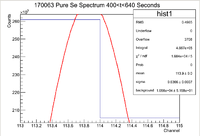
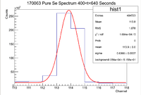
Here, the constant value is to assess the value for the background. The background must be removed from the signal in order to have a more accurate analysis as it is not a part of the signal that we are interested in. Below are sample plots of the original signal and the signal viewed in a thin 2 channel window:

This signal corresponds to the 103 keV line of Se-81. I plotted channel number instead of energy to maintain integer bins and avoid a picket fencing effect in the signal.

In looking at the thin window, the total number of counts within the window is given by the "Integral" value in the statistics box, which I will denote as I.

[math] Stats Box Integral = I [/math]

Since this is a counting experiment, the error in the signal will be given by

[math] \sigma_{I} = \sqrt{I} [/math]

Dealing With Background

Now that I have discussed how to get the number of counts along with the uncertainty in the number of counts, I will now discuss how to remove the background from a signal.

In the statistics box, there is a value called "background" which corresponds to the constant value in the fit function. To removed the background from the number of counts in the statistics box, we must integrate the "background" value across the region of interest. In other words

[math] Background = B = \int_{113}^{115} C d(Channel) = C(115-113) [/math]

Since the "background" value in the statistics box has an error with it and by integrating we are essentially just multiplying by a constant, so in this case

[math] \sigma_{B} = \int_{113}^{115}\sigma_{C} d(Channel) = \sigma_{C}(115-113) [/math]

Now that we have a value for the background along with its uncertainty, we can find the true signal of interest within the window. To find this use the relations

[math] True Signal = N = I - B [/math]

[math] \sigma_{N} = \sqrt{\sigma_{I}^2 + \sigma_{B}^2} [/math]

Now we have values for the number of counts without background along with the uncertainty in that value.

Decay During the Measurement

It is worth noting that since the half life of the sample is rather short that by measuring for roughly 5 minutes for each sample, the activity at the beginning of the measurement and the activity at the end are not the same. For example, if we assume some initial activity, then look at the activity after five minutes it will be slightly lower. In other words, assuming a run time of 300 seconds

[math] A = A_0 \times e^{-\lambda t} = A_0 \times e^{-\lambda \times 300} = 0.94 \times A_0[/math]

This shows that the activity drops by about 6 percent during a measurement of 5 minutes. To remedy this, one can use the fact that the measurement being made is actually integrating the true value of the activity over the time of the measurement. Or

[math] A_{Measure} = \frac{\int_{0}^{t}A_{True}\times e^{-\lambda t}dt}{t} [/math]

By integrating and solving for the true activity, we find that

[math] A_{True} = \frac{e^{\lambda t}\times A_{Measure}\times t \times \lambda}{e^{\lambda t} -1} [/math]

The error in this value is dominated by the error in the measured value, so the error in the true activity can be found by

[math] \sigma_{A_{True}} = \frac{t\times e^{\lambda t} \times \lambda \times \sigma_{A_{Measure}}}{e^{\lambda t}-1} [/math]

Dead Time

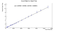
Dead time helps account for the number of counts that may have been lost because the data acquisition system was too busy recording. A count rate vs. % Dead time plot was made that is shown below:

Count Rate (Hz)	% Dead
129.47 +/- 7.84	0.24 +/- 0.10
154.33 +/- 10.36	0.29 +/- 0.11
194.83 +/- 8.36	0.41 +/- 0.11
253.69 +/- 14.05	0.51 +/- 0.18
257.11 +/- 11.24	0.53 +/- 0.14
338.8 +/- 11.68	0.65 +/- 0.15
477.61 +/- 15.06	0.84 +/- 0.16
619.3 +/- 10.56	1.34 +/- 0.18
680.83 +/- 17.5	1.33 +/- 0.23
807.37 +/- 15.85	1.55 +/- 0.18
889.6 +/- 16.22	1.65 +/- 0.34
1051.33 +/- 26.74	1.92 +/- 0.26
1213.93 +/- 23.62	2.26 +/- 0.33
1389.45 +/- 24.75	2.53 +/- 0.31
1628.47 +/- 17.17	3.06 +/- 0.30
2084.6 +/- 33.77	3.95 +/- 0.42
2576.5 +/- 31.53	5.06 +/- 0.39
3058.20 +/- 35.62	5.87 +/- 0.54
3362.13 +/- 23.12	6.59 +/- 0.43
4067.2 +/- 45.37	8.18 +/- 0.66
4564.37 +/- 61.94	9.09 +/- 0.60
5511.6 +/- 64.60	10.86 +/- 0.85

Below is a plot of the data

To account for the dead time, look at the total number of entries in the histogram and divide by the run time to get an average count rate. Then use the table to estimate the dead time. Once the dead time has been estimated, the correction factor is given by

[math] Dead Time Correction = \frac{1}{1-%Dead} [/math]