HRRL 03-17-2011

Good Tune Used for good Scan

By Dr. Kim

Solenoid 1	6.8 A
Solenoid 2	10.4 A
Gun Ver	-0.2 A
Gun Hor	+0.4 A
Output Hor	-1.4A
Output Ver	-0.5 A
Gun HV	+9.75 (Knob Setting)
Gun Grid Voltage	5.25 (Knob Setting)
RF frequency	2855.816 MHz
Modulator HV Power Supply	4.42 (Knob Setting)
RF macro Pulse Length (FWHM)	200 ns
Peak Current on FC	37.2 mAmps
Scope on FC
e- Beam Energy	14 MeV

Scan Description

This is scan for 14 MeV beam. 40 mAmps peak current. Q1 is on, All other quads are off.

1) Scan from -5 Amps to 5 Amps

2) Increment at 0.2 Amps.

3) Name images by numbers start from 1. Then go on.

Like: -5 Amp is 1, -4.8 Amp is 2, and so on til 5 Amp is named 51.

4) Scan multipole times from -5 to 5 Amps, and put them in different folders.

5) For each time, take back ground images. It should be done when RF is on and gun is off.

6) After the scan take a scope image for the current of the FC after the OTR screen.

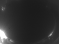
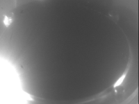
Calibration

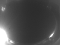
image	OTR image	cal_h (mm/px)	cal_v (mm/px)
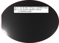		0.04308	0.04204
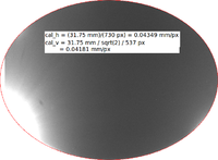		0.04320	0.04228
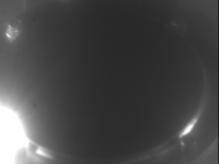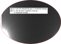		0.04349	0.04181
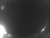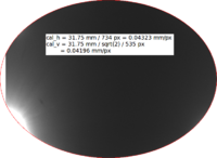		0.04323	0.04196
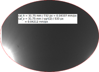		0.04337	0.04212
		mean (mm/px)	mean (mm/px)
		[math] 0.04327 \pm 0.00016 [/math]	[math] 0.04204 \pm 0.00018 [/math]

Results

Q1

At lower current background subtraction gets worse, because singal/noise drops.

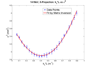
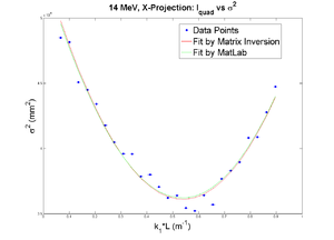
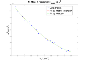
42 mA, Positive Current, X projection

emit=0.388 +- 0.008 mm*mrad, emit_norm=10.64 +- 0.22 mm*mrad

beta=1.285 +- 0.024, alpha=0.94 +-0.03

//K1*L(1/m)   er K1*L    sgima^2(mm)   er sigma^2

Media:2011_Mar_Emit_fit_data_x.txt

parabola fit for x-projection:

parabola fit for y-projection (y in mm unit):

y = (3.69167 +-0.02346) + (-3.89000+-0.12250)*x + (4.79738+-0.13309)*x.*x

Data created from parabola fit

Media:2011_Mar_Emit_data_from_fit_x.txt

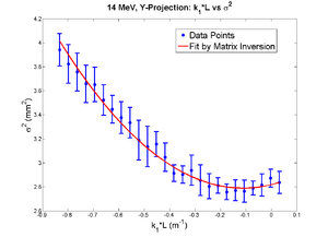
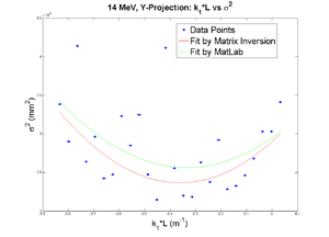
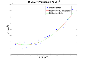
42 mA, Negative Current, Y projection

emit=0.266 +- 0.018 mm*mrad, emit_norm=7.30 +- 0.50 mm*mrad

beta=0.918 +- 0.068, alpha=0.19 +-0.06

//K1*L(1/m)   er K1*L    sgima^2(mm)   er sigma^2

Media:2011_Mar_Emit_fit_data_y.txt

parabola fit for y-projection (y in mm unit):

y = (2.81806 +-0.03890) + (0.52202+-0.26284)*x + (2.35025+-0.34553)*x.*x

Data created from parabola fit

Media:2011_Mar_Emit_data_from_fit_y.txt

X and Y emittances are different. The parabola in X reaches min around 0.4, while in Y reaches around 0.15. Which suggests quadrupole strengths of X and Y are way different for same coil current. Which might suggest beam is not centered, because when beam is off-centered we have this can occur.

20 mA, Positive Current, X projection

10 mA, Positive Current, X projection

5 mA, Positive Current, X projection

Q4

42 mA All Other Quads off

Haven't reach minimum.

42 mA Q1_at_-2A, Q2_at_+8A, Q3_at_-6A

x-projection:

y-projection:

Fits After the Second Mapping of the Quad

I mapped the quad to find effective length of the quad for different currents. Results are at: Second Mapping of Quadruple Magnets

MATLAB Scripts

Media:hrrl_2011_marc_emit_test_marc17_SuperGaussian_Fit.txt

Media:hrrl_2011_marc_emit_test_marc17_SupGau_devsum.txt

Media:hrrl_2011_marc_emit_test_marc17_Emit_Parabola_Fit_kl_XProjection.txt

Media:hrrl_2011_marc_emit_test_marc17_Emit_Parabola_Fit_kl_YProjection.txt

Media:hrrl_2011_marc_emit_test_marc17_Trial_my_superGaussian_Fit.txt

Media:hrrl_2011_marc_emit_test_marc17_Plot_Beam_Spot.txt

Media:hrrl_2011_marc_emit_test_marc17_Three_d_surface_plotter.txt

Media:hrrl_2011_marc_emit_test_marc17_my_superGaussian_Fit.txt

Media:hrrl_2011_marc_emit_test_marc17_devsum.txt

Media:hrrl_2011_marc_emit_test_marc17_countor_plotter.txt

With thin lens approximation method

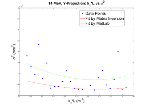
Why y projection has bigger error?

Quad was mapping for the second time to find effective length for the different currents. Link is at [[1]].

X

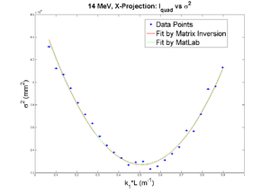
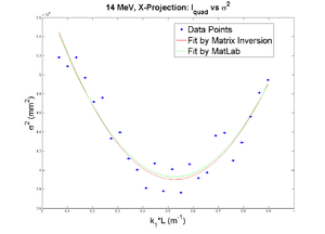
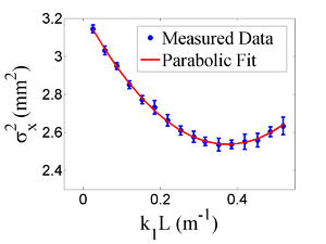
x-projection:

emit=0.417 +- 0.023 mm*mrad, emit_norm=11.43 +- 0.64 mm*mrad

beta=1.385 +- 0.065, alpha=0.97 +-0.07

parabola fit for x-projection (y in mm unit):

y = (3.67838 +-0.02232) + (-4.17265+-0.22057)*x + (5.55113+-0.42056)*x.*x

[math] \sigma_x^2= (3.678 \pm 0.022) + (-4.17 \pm 0.22)k_1L + (5.55 \pm 0.42)(k_1L)^2 [/math]

[math] \epsilon_x = 0.417 \pm 0.023~mm*mrad ~\Rightarrow~ \epsilon_{n,x} = 11.43 \pm 0.64~mm*mrad[/math]

[math] \beta_x=1.385 \pm 0.065, \alpha_x=0.97 \pm 0.07 [/math]

Y

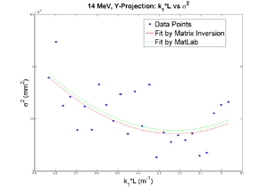
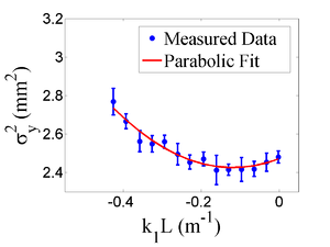
y-projection:

emit=0.338 +- 0.065 mm*mrad, emit_norm=9.25 +- 1.77 mm*mrad

beta=1.170 +- 0.192, alpha=0.22 +-0.10

parabola fit for y-projection (y in mm unit):

y = (2.84273 +-0.04370) + (1.02450+-0.51931)*x + (3.79913+-1.23728)*x.*x

[math]\sigma_y^2 = (2.843 \pm 0.044) + (1.02 \pm 0.52)k_1L + (3.8 \pm 1.2)(k_1L)^2 [/math]

[math] \epsilon_y = 0.338 \pm 0.065~mm*mrad ~\Rightarrow~ \epsilon_{n,y} = 9.3 \pm 1.8~mm*mrad[/math]

[math] \beta_y=1.17 \pm 0.19, \alpha_y=0.22 \pm 0.10 [/math]

Without thin lens approximation method

Thin lens approximation holds when [math] \sqrt{k_1}\times L_{QM} \lt \lt 1[/math] is true.

In our case [math] \sqrt{k_{1}} \times L_{QM} = \sqrt{0.5} \times 0.1 = 0.07 \lt 1 [/math]

HRRL_Emittance_Measurements_March14-18-2011