Difference between revisions of "05/13/2011 timing test"
Jump to navigation
Jump to search
| Line 38: | Line 38: | ||
Below is the plot of measured time as function of distances: | Below is the plot of measured time as function of distances: | ||
| + | |||
| + | {| border="0" cellspacing="0" style="text-align: center; width: 1050px; height: 100px;" | ||
| + | |[[File:Timing 1 10.png | 500px]] || [[File:Timing 11 30.png | 500px]] | ||
| + | |- | ||
| + | !colspan="6" | File:Timing 1 30.png | ||
| + | |} | ||
| + | |||
| + | |||
[[File:Timing 03.png | 800px]] | [[File:Timing 03.png | 800px]] | ||
Revision as of 04:03, 17 May 2011
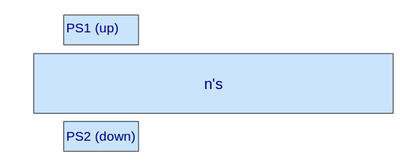
Set up like that:
The voltages, thresholds and widths are:
| PMT voltage, V | threshold, mV | discr. width, ns | |
|---|---|---|---|
| PS1 | -1000 | -80 | 50 |
| PS1 | -1000 | -80 | 50 |
| n's | -1500 | -200 | 10 |
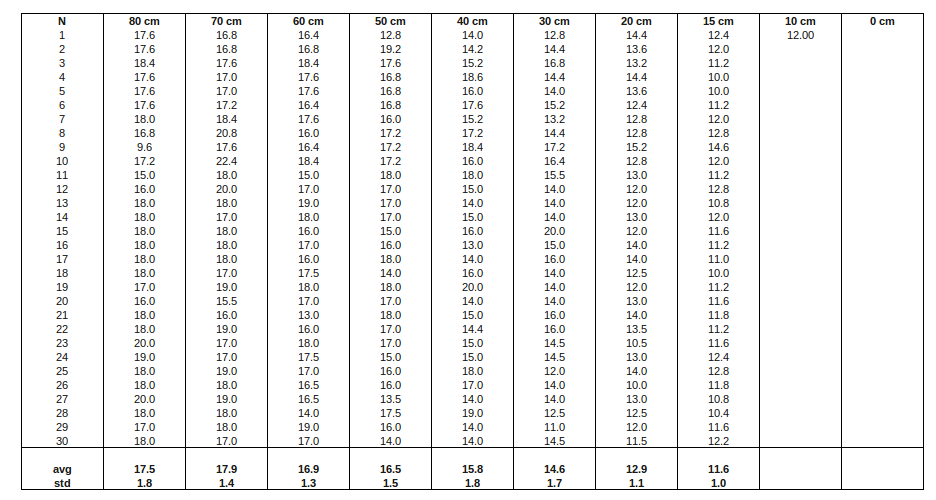
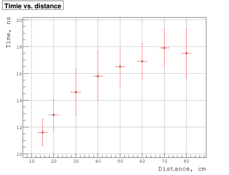
Let's do the timing test. The distances are between PS1+PS2 and n's PMT. The time is time difference between PS1(PS2) and n's detector signals
As the distance becomes 10 cm and less the coincidence rate becomes very low. I have:
- ▫ 11 coincidence for 98 min (10 cm)
- ▫ 0 coincidence for 10 min
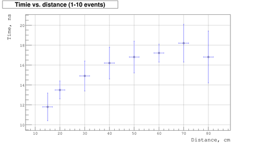
Below is the plot of measured time as function of distances:
 |
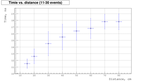
| ||||
| File:Timing 1 30.png | |||||
|---|---|---|---|---|---|
