Difference between revisions of "Se170063 Nickel Foil Thin Gauss Window Expansion"
| Line 1: | Line 1: | ||
| − | This analysis was done by weighting the histogram by the mass of the sample. The window is [1360,1365] and was expanded by one channel on each side to find the error in the counts. | + | This analysis was done by weighting the histogram by the mass of the sample. The window is [1360,1365] and was expanded by one channel on each side to find the error in the counts. Since the window is smaller, a constant fit was no long acceptable as the constant kept becoming negative and would yield a negative integral, which is not a good representation of background that is clearly there. Instead I used a linear function plus a gaussian to fit, then integrated the line across the window. |
{| border="3" cellpadding="5" cellspacing="0" | {| border="3" cellpadding="5" cellspacing="0" | ||
|| || 5/25/17 || 5/26/17 || 5/27/17 || 5/29/17 || 5/30/17 || 5/31/17 || 6/1/17 | || || 5/25/17 || 5/26/17 || 5/27/17 || 5/29/17 || 5/30/17 || 5/31/17 || 6/1/17 | ||
|- | |- | ||
| − | ||Original Window Counts || | + | ||Original Window Counts || |
|- | |- | ||
| − | || Original Window Background (Integrated) || | + | || Original Window Background (Integrated) || |
|- | |- | ||
| − | ||Original Window Difference || | + | ||Original Window Difference || |
|- | |- | ||
| − | ||Expanded Window Counts || | + | ||Expanded Window Counts || |
|- | |- | ||
| − | ||Expanded Window Background || | + | ||Expanded Window Background || |
|- | |- | ||
| − | ||Expanded Window Difference || | + | ||Expanded Window Difference || |
|- | |- | ||
| − | ||Error in counts || | + | ||Error in counts || |
|- | |- | ||
||Position || 50 cm || 30 cm ||20cm || 20 cm || 10cm || 10cm || 10cm | ||Position || 50 cm || 30 cm ||20cm || 20 cm || 10cm || 10cm || 10cm | ||
| Line 22: | Line 22: | ||
||Efficiency || 0.00017 || 0.000422 || 0.000847 || 0.000847 || 0.0031 || 0.0031 || 0.0031 | ||Efficiency || 0.00017 || 0.000422 || 0.000847 || 0.000847 || 0.0031 || 0.0031 || 0.0031 | ||
|- | |- | ||
| − | ||.dat file entry || | + | ||.dat file entry || |
|- | |- | ||
|} | |} | ||
Revision as of 14:41, 26 October 2017
This analysis was done by weighting the histogram by the mass of the sample. The window is [1360,1365] and was expanded by one channel on each side to find the error in the counts. Since the window is smaller, a constant fit was no long acceptable as the constant kept becoming negative and would yield a negative integral, which is not a good representation of background that is clearly there. Instead I used a linear function plus a gaussian to fit, then integrated the line across the window.
| 5/25/17 | 5/26/17 | 5/27/17 | 5/29/17 | 5/30/17 | 5/31/17 | 6/1/17 | |
| Original Window Counts | |||||||
| Original Window Background (Integrated) | |||||||
| Original Window Difference | |||||||
| Expanded Window Counts | |||||||
| Expanded Window Background | |||||||
| Expanded Window Difference | |||||||
| Error in counts | |||||||
| Position | 50 cm | 30 cm | 20cm | 20 cm | 10cm | 10cm | 10cm |
| Efficiency | 0.00017 | 0.000422 | 0.000847 | 0.000847 | 0.0031 | 0.0031 | 0.0031 |
| .dat file entry |
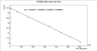
Below is a plot of the activity as a function of time
This gives the constant of 14.5046 +/- 0.00345043. Now find the initial activity
Since the plot is made with reference to the mixture's measurement time (first point plotted 108 minutes after the mix was measured) means that the constant should be the activity at the time the mixture was being measured.
