Wire angle correspondance

Determining wire-theta correspondance

To associate the hits with the Moller scattering angle theta, the occupancy plots of the drift chamber hits by means of wire numbers and layer must be translated using the physical constraints of the detector. Using the data released for the DC:

DC: Drift Chambers(specs)

This gives the detector with a working range of 5 to 40 degrees in Theta for the lab frame, with a resolution of 1m radian.

This sets the lower limit:

$\frac{5^{\circ}}{1}\frac{\pi\ radians}{180^{\circ}}=.0872664626\ radians$

This sets the upper limit:

$\frac{40^{\circ}}{1}\frac{\pi\ radians}{180^{\circ}}=.698131700798\ radians$

Taking the difference,

$.698131700798-.0872664626\approx\ .61086523198\ radians$

Dividing by 112, we find

$\frac{.61086523198}{112}=.005454153912\ radians\approx\ 0.0055\ radians$

CED Verification

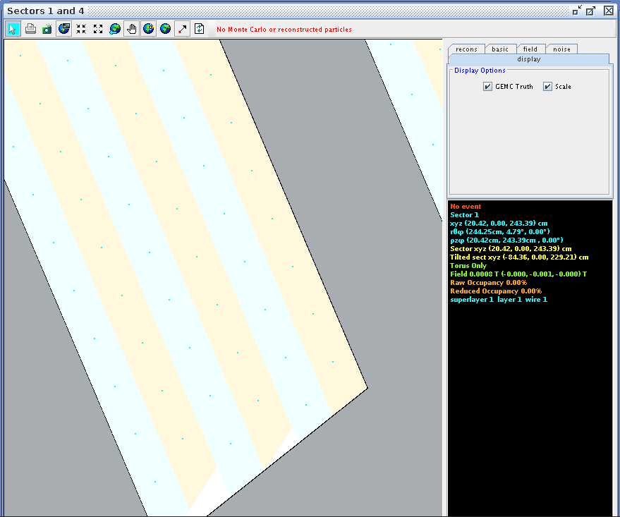
Using CED to verify the angle and wire correlation,

Zooming in on the view paralell to the direction of the wires in ced, we can examine the wire corresponding theta angle in the drift chamber.

Corresponding theta angles can be found for other wires, in Region 1, Superlayers 1 and 2.

Table 1: Superlayer 1 Wire-Angle Theta Correspondence in Degrees

Wire Number	Layer 1	Layer 2	Layer 3	Layer 4	Layer 5	Layer 6
1	4.79	5.03	4.98	5.22	5.16	5.40
2	5.09	5.33	5.27	5.51	5.45	5.69
78	29.79	29.93	29.74	29.88	29.69	29.83
111	40.50	40.59	40.36	40.44	40.21	40.29
112	40.82	40.90	40.67	40.75	40.52	40.60

Table 2: Superlayer 2 Wire-Angle Theta Correspondence in Degrees

Wire Number	Layer 1	Layer 2	Layer 3	Layer 4	Layer 5	Layer 6
1	4.79	5.03	4.98	5.22	5.16	5.40
2	5.09	5.33	5.27	5.51	5.45	5.69
78	29.79	29.93	29.74	29.88	29.70	29.84
111	40.51	40.59	40.36	40.44	40.22	40.30
112	40.82	40.90	40.67	40.75	40.52	40.60

Super Layer 1:Layer 1

Finding the difference between wires 1 and 2,

$\frac{5.09^{\circ}-4.79^{\circ} }{wire\ number}=\frac{.3^{\circ}}{wire\ number}$

Finding the difference between wires 111 and 112,

$\frac{40.82^{\circ}-40.50^{\circ}}{wire\ number}=\frac{.32^{\circ}}{wire\ number}$

Examing the range limits for the angle theta:

Taking the difference of the upper and lower limits in theta,

$40.82^{\circ}-4.79^{\circ}=36.03^{\circ}$

Dividing by 112 wires, we find

$\frac{36.03^{\circ}}{112\ wires}\approx\ \frac{0.322^{\circ}}{wire\ number}$

Changing cell size

Using Mathematica, a line can be fitted to the data collected on the wire number to angle theta correspondence.

Declaring the data set:

In[1]:= data1={{1,4.79},{2,5.09},{78,29.79},{111,40.50},{112,40.82}}

Out[1]= {{1,4.79},{2,5.09},{78,29.79},{111,40.5},{112,40.82}}

Testing for a linear fit:

In[2]:= line1=Fit[data1,{1,x},x]

Out[2]= 4.69004 +0.323914 x

Testing for a quadratic fit:

In[3]:= quad1=Fit[data1,{1,x,x^2},x]

Out[3]= 4.69669 +0.322347 x+0.0000143086 x^2

Testing for a polynomial of degree 3 fit:

In[4]:= polynomial1=Fit[data1,{1,x,x^2,x^3},x]

Out[4]= 4.65523 +0.351087 x-0.000597139 x^2+3.20201*10^-6 x^3