Difference between revisions of "Simulations of Particle Interactions with Matter"
| Line 274: | Line 274: | ||
We can use the above relationships to construct a Hamilton in terms of <math>\vec{r}</math> instead of <math>\vec{r_1}</math> and <math> \vec{r_2}</math> thereby reducing the problem from a 2-body problem to a 1-body problem. | We can use the above relationships to construct a Hamilton in terms of <math>\vec{r}</math> instead of <math>\vec{r_1}</math> and <math> \vec{r_2}</math> thereby reducing the problem from a 2-body problem to a 1-body problem. | ||
| + | |||
| + | ; Construct the Hamiltonian | ||
| + | |||
| + | To construct the Hamiltonian for this problem we will start with the Lagrangian. | ||
| + | |||
| + | |||
| + | <math>\cal{L} = T - U</math> | ||
| + | |||
| + | where | ||
| + | |||
| + | <math>T \equiv</math> kinetic energy of the system | ||
| + | <math>U \equiv</math> Potential energy of the system | ||
==== Lab Frame Cross Sections ==== | ==== Lab Frame Cross Sections ==== | ||
Revision as of 20:45, 5 September 2007
Overview
Particle Detection
A device detects a particle only after the particle transfers energy to the device.
Energy intrinsic to a device depends on the material used in a device
Some device of material with an average atomic number () is at some temperature (). The materials atoms are in constant thermal motion (unless T = zero degrees Klevin).
Statistical Thermodynamics tells us that the canonical energy distribution of the atoms is given by the Maxwell-Boltzmann statistics such that
represents the probability of any atom in the system having an energy where
Note: You may be more familiar with the Maxwell-Boltzmann distribution in the form
where would represent the molesules in the gas sample with speeds between and
Example 1: P(E=5 eV)
- What is the probability that an atom in a 12.011 gram block of carbon would have and energy of 5 eV?
First lets check that the probability distribution is Normailized; ie: does ?
is calculated by integrating P(E) over some energy interval ( ie:). I will arbitrarily choose 4.9 eV to 5.1 eV as a starting point.
assuming a room empterature of
then
and
or in other words the precise mathematical calculation of the probability may be approximated by just using the distribution function alone
This approximation breaks down as
Since we have 12.011 grams of carbon and 1 mole of carbon = 12.011 g = carbon atoms
We do not expect to see a 5 eV carbon atom in a sample size of carbon atoms when the probability of observing such an atom is
The energy we expect to see would be calculated by
If you used this block of carbon as a detector you would easily notice an event in which a carbon atom absorbed 5 eV of energy as compared to the energy of a typical atom in the carbon block.
- Silicon detectors and Ionization chambers are two commonly used devices for detecting radiation.
approximately 1 eV of energy is all that you need to create an electron-ion pair in Silicon
approximately 10 eV of energy is needed to ionize an atom in a gas chamber
The low probability of having an atom with 10 eV of energy means that an ionization chamber would have a better Signal to Noise ratio (SNR) for detecting 10 eV radiation than a silicon detector
But if you cool the silicon detector to 200 degrees Kelvin (200 K) then
So cooling your detector will slow the atoms down making it more noticable when one of the atoms absorbs energy.
also, if the radiation flux is large, more electron-hole pairs are created and you get a more noticeable signal.
Unfortunately, with some detectore, like silicon, you can cause radiation damage that diminishes it's quantum efficiency for absorbing energy.
The Monte Carlo method
- Stochastic
- from the greek word "stachos"
- a means of, relating to, or characterized by conjecture and randomness.
A stochastic process is one whose behavior is non-deterministic in that the next state of the process is partially determined.
Physics has many such non-deterministic systems:
- Quantum Mechanics
- Thermodynamics
Basically the monte-carlo method uses a random number generator (RNG) to generate a distribution (gaussian, uniform, Poission,...) which is used to solve a stochastic process based on an astochastic description.
Example 2 Calculation of
- Astochastic description
- may be measured as the ratio of the area of a circle of radius divided by the area of a square of length
You can measure the value of if you physically measure the above ratios.
- Stochastic description
- Construct a dart board representing the above geometry, throw several darts at it, and look at a ratio of the number of darts in the circle to the total number of darts thrown (assuming you always hit the dart board).
- Monte-Carlo Method
- Here is an outline of a program to calulate using the Monte-Carlo method with the above Stochastic description
begin loop
 x=rnd
 y=rnd
 dist=sqrt(x*x+y*y)
 if dist <= 1.0 then numbCircHits+=1.0
 numbSquareHist += 1.0
end loop
 print PI = 4*numbCircHits/numbSquareHits
A Unix Primer
To get our feet wet using the UNIX operating system, we will try to solve example 2 above using a RNG under UNIX
List of important Commands
- ls
- pwd
- cd
- df
- ssh
- scp
- mkdir
- printenv
- emacs, vi, vim
- make, gcc
- man
- less
- rm
Most of the commands executed within a shell under UNIX have command line arguments (switches) which tell the command to print information about using the command to the screen. The common forms of these switches are "-h", "--h", or "--help"
ls --help
ssh -h
the switch deponds on your flavor of UNIX
if using the switch doesn;t help you can try the "man" (sort for manual) pages (if they were installed). Try
man -k pwd
the above command will search the manual for the key word "pwd"
Example 3: using UNIX
Step
- login to inca.
click here for a description of logging in if using windows - mkdir src
- cd src
- cp -R ~tforest/NucSim/Day1 ./
- ls
- cd Day1
- make
- ./rndtest
Here is a web link to the source files you can copy in case the above doesn't work
A Root Primer
Example 1: Create Ntuple and Draw Histogram
Cross Sections
Definitions
= scattering cross-section
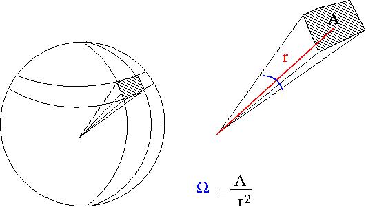
- Solid Angle

- = surface area of a sphere covered by the detector
- ie;the detectors area projected onto the surface of a sphere
- A= surface area of detector
- r=distance from interaction point to detector
- sterradians
- if your detector was a hollow ball
- sterradians
- Units
- Cross-sections have the units of Area
- 1 barn =
- [units of ] =
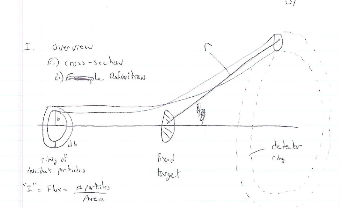
- Fixed target scattering
- = # of particles in =
- is the area of the ring of incident particles
- = # particles in a ring of radius and thickness
You can measure if you measure the # of particles detected in a known detector solid angle from a know incident particle Flux () as
Alternatively if you have a theory which tells you which you want to test experimentally with a beam of flux then you would measure counts (particles)
- Units
- = # of particles
- or for a count rate divide both sides by time and you get beam current on the RHS
- integrate and you have the total number of counts
- Classical Scattering
- In classical scattering you get the same number of particle out that you put in (no capture, conversion,..)
- tells you how the impact parameter changes with scattering angle
Example : Elastic Scattering
This example is an example of classical scattering.
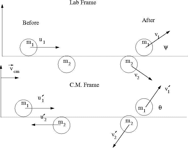
Our goal is to find for an elastic collision of 2 impenetrable spheres of diameter . To solve this elastic scattering problem we will describe the collision in the Center of Mass (C.M.) frame. As we shall see, in the C.M. fram the 2-body collision becomes a 1-body problem.
- Variable definitions
- = impact parameter ; distance of closest approach
- = mass of incoming ball
- = mass of target ball
- = iniital velocity of incoming ball in Lab Frame
- = final velocity of in Lab Frame
- = scattering angle of in lab frame after collision
- = iniital velocity of in C.M. Frame
- = final velocity of in C.M. Frame
- = iniital velocity of in C.M. Frame
- = final velocity of in C.M. Frame
- = scattering angle of in C.M. frame after collision
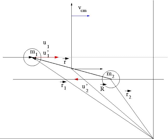
We can reduct the 2-body problem to a 1-body problem using the following coordinates
- vector definitions
- = a position vector pointing to the location of
- = a position vector pointing to the location of
- = a position vector pointing to the center of mass of the two ball system
- = the magnitude of this vector is the distance between the two masses
In the C.M. reference frame the above vectors have the following relationships
solving the above equations for and and defining the reduced mass as
- reduced mass
leads to
We can use the above relationships to construct a Hamilton in terms of instead of and thereby reducing the problem from a 2-body problem to a 1-body problem.
- Construct the Hamiltonian
To construct the Hamiltonian for this problem we will start with the Lagrangian.
where
kinetic energy of the system Potential energy of the system


