|
|
| Line 57: |
Line 57: |
| | For an incoming electron with momentum of 11GeV, we should find the momentum in the center of mass to be around '''53 MeV''' which is confirmed in the the data/plots. | | For an incoming electron with momentum of 11GeV, we should find the momentum in the center of mass to be around '''53 MeV''' which is confirmed in the the data/plots. |
| | | | |
| − | ===Simulation Verification===
| |
| − | Sample output from GEANT4 simulation:
| |
| − |
| |
| − |
| |
| − | {| border=1
| |
| − | |-
| |
| − | ! KE<sub>i</sub> !! Px<sub>i</sub> !! Py<sub>i</sub> !! Pz<sub>i</sub> !! x<sub>i</sub> !! y<sub>i</sub> !! z<sub>i</sub> !! KE<sub>f</sub> !! Px<sub>f</sub> !! Py<sub>f</sub> !! Pz<sub>f</sub> !! x<sub>f</sub> !! y<sub>f</sub> !! z<sub>f</sub> !! KE<sub>m</sub> !! Px<sub>m</sub> !! Py<sub>m</sub> !! Pz<sub>m</sub> !! x<sub>m</sub> !! y<sub>m</sub> !! z<sub>m</sub>
| |
| − | |-
| |
| − | | 11000 || 0 || 0 || 11000.5 || 0 || 0 || -510 || 10999.1 || 0.433025 || -0.858867 || 10999.6 || 0 || 0 || -509.276 || 0.905324 || -0.433025 || 0.858867 || 0.905366 || 0 || 0 || -509.276
| |
| − | |}
| |
| − |
| |
| − |
| |
| − | Running a GEANT simulation just to put this set into a .dat file, then using the .dat file through the Moller_OG.C file in ROOT, we find in the Lab Frame:
| |
| − |
| |
| − |
| |
| − |
| |
| − | Fnl4Mom.P 10999.599651
| |
| − | Fnl4Mom.E 10999.610609
| |
| − | Mol4Mom.P 1.320928
| |
| − | Mol4Mom.E 1.416324
| |
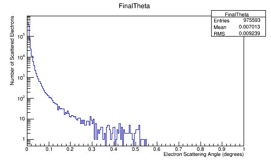
| − | Fnl4Mom.Theta(degrees) 0.005013
| |
| − | Fnl4Mom.Theta(radians) 0.000087
| |
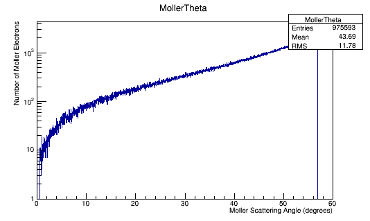
| − | Mol4Mom.Theta(degrees) 46.756514
| |
| − | Mol4Mom.Theta(radians) 0.815641
| |
| − |
| |
| − | Fnl4Mom.P 52.455386
| |
| − | Fnl4Mom.E 54.704969
| |
| − | Mol4Mom.P 52.455386
| |
| − | Mol4Mom.E 52.457875
| |
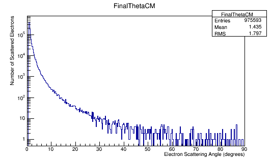
| − | Fnl4Mom.Theta(degrees) 1.051202
| |
| − | Fnl4Mom.Theta(radians) 0.018338
| |
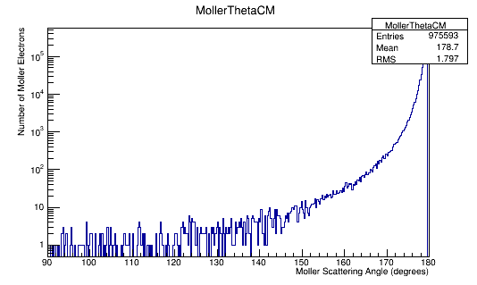
| − | Mol4Mom.Theta(degrees) 179.040096
| |
| − | Mol4Mom.Theta(radians) 3.123255
| |
| − |
| |
| − |
| |
| − |
| |
| − | [[File:FnlMomCM.png]][[File:MolMomCM.png]]
| |
| − | ====Explaining graph distribution====
| |
| − |
| |
| − | Trying to explain the graphs, we look at the data files for strange KE, hence weirder momentums
| |
| − |
| |
| − |
| |
| − | {| border=1
| |
| − | |-
| |
| − | ! KE<sub>i</sub> !! Px<sub>i</sub> !! Py<sub>i</sub> !! Pz<sub>i</sub> !! x<sub>i</sub> !! y<sub>i</sub> !! z<sub>i</sub> !! KE<sub>f</sub> !! Px<sub>f</sub> !! Py<sub>f</sub> !! Pz<sub>f</sub> !! x<sub>f</sub> !! y<sub>f</sub> !! z<sub>f</sub> !! KE<sub>m</sub> !! Px<sub>m</sub> !! Py<sub>m</sub> !! Pz<sub>m</sub> !! x<sub>m</sub> !! y<sub>m</sub> !! z<sub>m</sub>
| |
| − | |-
| |
| − | | 11000 || 0 || 0 || 11000.5 || 0 || 0 || -510 || 9855.29 || -31.7166 || -6.48546 || 9855.75 || 0 || 0 || -501.365 || 1144.53 || 31.7166 || 6.48546 || 1144.59 || 0 || 0 || -501.365
| |
| − | |-
| |
| − | | 11000 || 0 || 0 || 11000.5 || 0 || 0 || -510 || 10999.0996 || -0.152974 || -0.761885 || 10999.7 || 0 || 0 || -502.19 || 0.590904 || 0.152974 || 0.761885 || 0.590932 || 0 || 0 || -502.191986
| |
| − | |}
| |
| − |
| |
| − |
| |
| − | =====Momentum below 53 MeV=====
| |
| − |
| |
| − | Using the equations derived earlier,
| |
| − |
| |
| − | <center><math>E_{cm}=(m_1^2+m_2^2+2E_{1 lab}m_2)^{1/2}</math></center>
| |
| − |
| |
| − |
| |
| − | <center><math>p_{cm}=\frac{p_{lab}m_2}{E_{cm}}</math></center>
| |
| − |
| |
| − | For the KE<sub>f</sub>=9855.29 MeV, we find that
| |
| − |
| |
| − | <center><math>E_{1 lab}=KE_f+.511\times 10^6=9855.29\times 10^6+.511\times 10^6=9.855\times 10^9 eV</math></center>
| |
| − |
| |
| − |
| |
| − | <center><math>p_{lab}=((-31.72\times 10^6)^2+(-6.48\times 10^6)^2+(9855.75\times 10^6)^2)^{1/2}=9.855\times 10^9 \frac{eV}{c}</math></center>
| |
| − |
| |
| − |
| |
| − | <center><math>E_{cm}=(m_1^2+m_2^2+2E_{1 lab}m_2)^{1/2}=((0.511\times 10^6)^2+(0.511\times 10^6)^2+2\times (9.855\times 10^3)\times 0.511\times 10^6)^{1/2}</math></center>
| |
| − |
| |
| − |
| |
| − | this gives
| |
| − |
| |
| − | <center><math>E_{cm}=1.00\times 10^8 eV</math></center>
| |
| − |
| |
| − |
| |
| − | <center><math>p_{cm}=\frac{p_{lab}m_2}{E_{cm}}=\frac{(9.855\times 10^9)\times (.511\times 10^6)}{1\times 10^8}=50 \frac{MeV}{c}</math></center>
| |
| − |
| |
| − | This explains the lower bound part of the graph in that some of the initial particles transfer a large amount of energy to the Moller electron.
| |
| − |
| |
| − | =====Momentum above 53 MeV=====
| |
| − | For the second set of data, simulation finds the boost to be
| |
| − |
| |
| − | {| border=1
| |
| − | |-
| |
| − | ! P<sub>cm</sub> !! Px<sub>cm</sub> !! Py<sub>cm</sub> !! Pz<sub>cm</sub> !! E<sub>cm</sub>
| |
| − | |-
| |
| − | | 58.379341 || -0.152974 || -0.761885 || 58.374168 || 37.904019
| |
| − | |}
| |
| − |
| |
| − | Using the approximation used above doesn't give the Energy in the Center of Mass as 58 MeV, it yields 53 MeV. Maybe the 2nd electron isn't initially at rest? Using the other form,
| |
| − |
| |
| − |
| |
| − | <center><math>E_{cm}=((E_{1 lab}+E_{2 lab})^2-(\vec{p}_{1 lab}+\vec{p}_{2 lab})^2)^{1/2}</math></center>
| |
| − |
| |
| − |
| |
| − | <center><math>E_{cm}=(((10999.0996\times 10^6+.511\times 10^6)+(0.590904\times 10^6+.511\times 10^6))^2-(1.09997000\times 10^{10}+9.76253259\times 10^5)^2)^{1/2}</math></center>
| |
| − |
| |
| − |
| |
| − | <center><math>E_{cm}=(1.21015675596\times 10^{20}-1.21014878029\times 10^{20})^{1/2}</math></center>
| |
| − |
| |
| − |
| |
| − | <center><math>E_{cm}=(7.97567\times 10^{14})^{1/2}=2.82\times 10^7</math></center>
| |
| − |
| |
| − | Rounding choices can greatly alter the value obtained.
| |
| | | | |
| | Changing the code for the total Energy to <math>E=(p_1^2+m_1^2)^{1/2}</math> in the lab frame gives | | Changing the code for the total Energy to <math>E=(p_1^2+m_1^2)^{1/2}</math> in the lab frame gives |
Simulating the Moller scattering background for EG1
Step 1
Determine the Moller background using an LH2 target to check the physics in GEANT4
Incident electron energy varies from 1-11 GeV.
LH2 target is a cylinder with a 1.5 cm diameter and 1 cm thickness.
(Following dimensions listed on page 8 of File:PHY02-33.pdf)
Numbers Moller electrons per incident electron.
While 2nd and 3rd generations are created, only 2 2nd generation daughter particles are created for 1E6 incident particles. All knock on electrons are not counted.
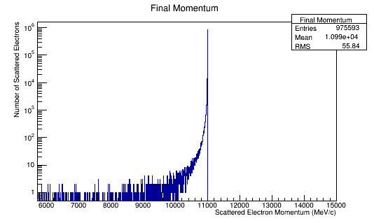
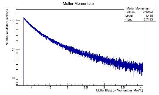
Estimated Momentum Distribution
In the collision of two particles of mass m_1 and m_2, the total energy in the center of mass frame can be written
[math]E_{cm}=((E_{1lab}+E_{2lab})^2-(\vec{p}_{1lab}+\vec{p}_{2lab})^2)^{1/2}[/math]
[math]E_{cm}=(m_1^2+m_2^2+2E_1E_2(1-\beta_1\beta_2cos\theta))^{1/2}[/math]
where θ is the angle between the particles.
In the frame where one particle (m2) is at rest
[math]E_{cm}=(m_1^2+m_2^2+2E_{1_{initial} lab}m_2)^{1/2}[/math]
where [math]E_{1_{initial} lab}=KE_{1 lab}+m_1[/math] in MeV
The velocity of the center of mass in the lab frame is
[math]\beta_{cm}=\frac{p_{lab}}{(E_{1 lab}+m_2)}[/math]
where plab≡p1 lab and
[math]\gamma_{cm}\frac{(E_{1_{initial} lab}+m_2)}{E_{cm}}[/math]
This gives the momenta of the particles in the center of mass to have equal magnitude, but opposite directions
[math]p_{cm}=\frac{p_{1_{initial}lab}m_2}{E_{cm}}[/math]
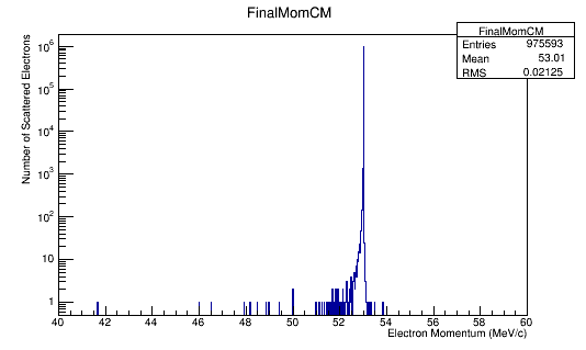
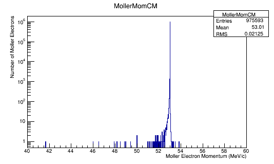
For an incoming electron with momentum of 11GeV, we should find the momentum in the center of mass to be around 53 MeV which is confirmed in the the data/plots.
Changing the code for the total Energy to [math]E=(p_1^2+m_1^2)^{1/2}[/math] in the lab frame gives
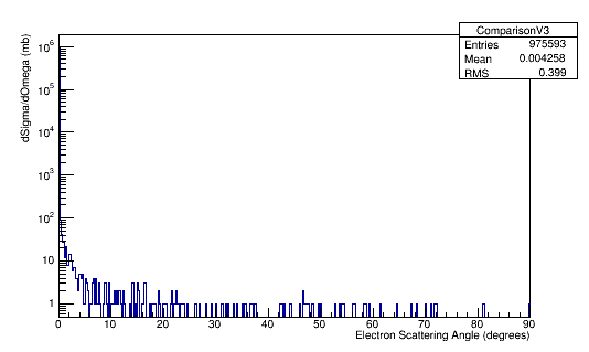
Angular Distribution in the Lab Frame
Angular Distribution in the Center of Mass Frame
Comparing experimental vs. theoretical for Møller differential cross section 11GeV
Using the equation from Halzen and Martin (p121) to approximate Moller scattering (in the Center of Mass Frame)
[math]\frac{d\sigma}{d\Omega}=\frac{m^2 \alpha^2}{16 p^4}\left(\frac{1}{\sin^4 \frac{\theta}{2}}+\frac{1}{\cos^4 \frac{\theta}{2}}-\frac{1}{\sin^2 \frac{\theta}{2}\cos^2 \frac{\theta}{2}}\right)[/math]
where [math]\alpha = \frac{1}{137}[/math]
Plugging in the values expected for a scattering electron:
[math]m^2 = \frac{(.000511 GeV)^2}{c^4}=2.6\times 10^{-7} GeV^2/c^4[/math]
[math]\alpha^2=\frac{1}{137^2}=7.3\times 10^{-3}[/math]
[math]p^4=\frac{(.053 GeV)^4}{c^4}=7.9\times 10^{-6} GeV^4/c^4[/math]
Using unit analysis on the term outside the parantheses, we find that the differential cross section for an electron at this momentum should be around
[math]\frac{m^2 \alpha^2}{16 p^4}=\frac{1.5\times 10^{-5}}{ GeV^{2}}[/math]
Using the conversion of
[math]\frac{1}{1GeV^{2}}=.3892 mb [/math]
We find that the differential cross section is [math]5.8\times 10^{-6} mb=5.8 nb[/math]
Converting the number of electrons to barns,
- [math]L=\frac{i_{scattered}}{\sigma} \approx i_{scattered}\times \rho_{target}\times l_{target}[/math]
where ρtarget is the density of the target material, ltarget is the length of the target, and iscattered is the number of incident particles scattered.
- [math]L=\frac{70.85 kg}{1 m^3}\times \frac{1 mole}{2.02 g} \times \frac{1000g}{1 kg} \times \frac{6\times10^{23} atoms}{1 mole} \times \frac{1cm}{100 cm} \times \frac{1 m}{ } \times \frac{10^{-23} m^2}{barn} =2.10\times 10^{-2} barns[/math]
- [math]\frac{1}{L \times 4\times 10^7}=1.19\times 10^{-6} barns[/math]
Step 2
Replace the LH2 target with an NH3 target and compare with LH2 target.
Step 3
Determine impact of Solenoid magnet on Moller events
Papers used
A polarized target for the CLAS detectorFile:PHY02-33.pdf
An investigation of the spin structure of the proton in deep inelastic scattering of polarized muons on polarized protons File:1819.pdf
EG12


