Difference between revisions of "HRRL 03-18-2011"

From New IAC Wiki
Jump to navigation Jump to search
Line 338: Line 338:
  
  
 +
== Super Gaussian Fitting ==
  
 +
Beam_Distribution_Beyond_RMS: [[File:Beam_Distribution_Beyond_RMS.pdf]]
 +
 +
Basic MATLAB Codes to fit Super Gaussian:
 +
 +
[[File:Trial_my_Super_Gaussian_fit.txt]]
 +
 +
[[File:SupGau_desum.txt]]
 +
 +
My MATLAB Fit code for beam
 +
 +
[[File:my_Super_Gaussian_fit.txt]]
 +
 +
[[File:SupGau_desum.txt]]
 +
 +
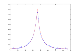
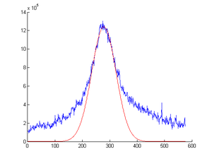
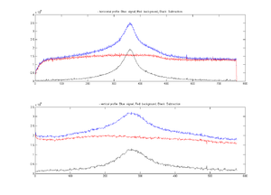
Here is an example fitting:
 +
 +
{| border="1"
 +
| Signal || Background || fit
 +
|-
 +
| [[File:HRRL_03-18-2011_Lorentzian_Fitting_Example_sg.png| 300 px]] || [[File:HRRL_03-18-2011_Lorentzian_Fitting_Example_bg.png| 300 px]]  || [[File:HRRL_03-18-2011_SupGau_Fitting_Example_1.png| 300 px]]
 +
|-
 +
| height of the peak || location of the peak ||  base
 +
|-
 +
| 8.0480e+003 || 359.6730 ||  201.9112
 +
|-
 +
| sigma_0 || N ||  sigma
 +
|-
 +
| 20.9204 || 0.8494 ||  38.5672
 +
|}


Revision as of 16:43, 7 April 2011

Tune parameters

Previous Tune at the higher energy

Solenoid 1 5.4 A
Solenoid 2 5.5 A
Gun Ver -0.2 A
Gun Hor +0.4 A
Output Hor -0.5 A
Output Ver -0.5 A
Gun HV +9.75 (Knob Setting)
Gun Grid Voltage 5.25 (Knob Setting)
RF frequency 2855.813 MHz
Modulator HV Power Supply 4.11 (Knob Setting)
RF macro Pulse Length (FWHM) 200 ns

Solenoid comparison with yesterdays higher energy tune

V1 (Gun Vertical) H1 (Gun Horizontal) Sol1 (Gun Sol) V2 (Output Vertical) H2 (Output horizontal Sol 2 (Output solenoid) OTR Pict FC pict
(A) (A) (A) (A) (A) (A)
(-0.3) +0 0 0 -0 -0 OTR Q1Scan03182011 SterOff.png FC Q1Scan03182011 SterOff.png
(-0.2) +0.4 5.4 -0.5 -0.5 5.5 OTR Q1Scan03182011 SterOn.png FC Q1Scan03182011 SterOon.png
(-0.2) +0.4 6.8 -0.5 -0.5 5.5 OTR Q1Scan03182011 1.png FC Q1Scan03182011 1.png
(-0.2) +0.4 6.8 -0.5 -0.5 10.4 OTR Q1Scan03182011 2.png FC Q1Scan03182011 2.png

Quad Scans

To test reproducibility from yesterday. Scan at 40, 20, 10, 5 mA peak currents. Scan twice on each Current.

Do Energy Scan

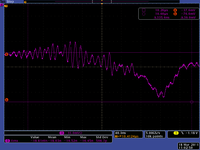
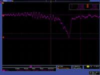
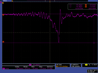
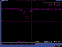
Bend the beam through 45 bending dipole, take images on the scope of FC and YAG images.

D1 current Energy FC peak Volt Pic
(A) MeV mV
28 11.85 39 FC2 0318011 28A 11.85.png
29 12.3 74 FC2 0318011 28A 12.3.png
30 12.74 93 FC2 0318011 30A 12.74.png
30.5 12.96 65 FC2 0318011 30.5A 12.96.png
30.7 large uncertainty 22 FC2 0318011 30.7A.png

Quad 1 Scan

Quad 1 OTR Pict FC pict
(A)
+0 OTR Q1Scan03182011 10.png FC Q1Scan03182011 10.png
+0.2 OTR Q1Scan03182011 11.png FC Q1Scan03182011 11.png
+0.4 OTR Q1Scan03182011 12.png FC Q1Scan03182011 12.png
+0.6 OTR Q1Scan03182011 13.png FC Q1Scan03182011 13.png
+0.8 OTR Q1Scan03182011 14.png FC Q1Scan03182011 14.png
+1.0 OTR Q1Scan03182011 15.png FC Q1Scan03182011 15.png
+1.2 OTR Q1Scan03182011 16.png FC Q1Scan03182011 16.png
+1.4 OTR Q1Scan03182011 17.png FC Q1Scan03182011 17.png
+1.6 OTR Q1Scan03182011 18.png FC Q1Scan03182011 18.png
+1.8 OTR Q1Scan03182011 19.png FC Q1Scan03182011 19.png
+2.0 OTR Q1Scan03182011 20.png FC Q1Scan03182011 20.png

Scan Quad 4

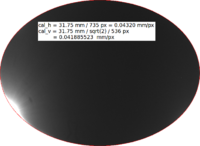
Calibration

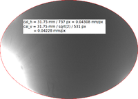
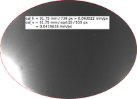
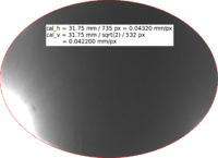
Estimate the error in the above calibration


image OTR image Calibration
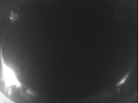
HRRL 03-18-2011 cal 1 source.png HRRL 03-18-2011 cal 1.png cal_h = 31.75 mm / 737 px = 0.04308 mm/px; cal_v = 31.75 mm / sqrt(2) / 531 px = 0.04228 mm/px;
HRRL 03-18-2011 cal 2 source.png HRRL 03-18-2011 cal 2.png cal_h = 31.75 mm / 738 px = 0.04302 mm/px; cal_v = 31.75 mm / sqrt(2) / 535 px = 0.04196 mm/px;
HRRL 03-18-2011 cal 3 source.png HRRL 03-18-2011 cal 3.png cal_h = 31.75 mm / 735 px = 0.04320 mm/px; cal_v = 31.75 mm / sqrt(2) / 532 px = 0.04220 mm/px;
HRRL 03-18-2011 cal 4 source.png HRRL 03-18-2011 cal 4.png cal_h = 31.75 mm / 735 px = 0.04320 mm/px; cal_v = 31.75 mm / sqrt(2) / 536 px = 0.04189 mm/px;

Data Analysis

Preliminary results

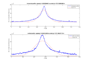
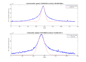
Here is the study on how to fit non_Gaussian curve. I fitted for whole image as well as parts of the image.

Here is beam profile, which is non-Gaussian.

Fits for whole image:

HRRL 03-18-2011 Data Analysis Preliminary Results non-Gauss profile 1.png

Fits for x=[362,404] and y=[241,301]:

HRRL 03-18-2011 Data Analysis Preliminary Results non-Gauss profile 2.png


Gaussian fitted for whole image

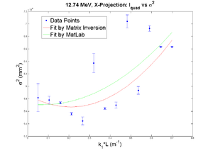
12.74 MeV

Fitted Gaussian for whole image x-projection:

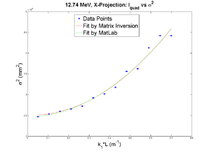
emit=0.521 +- 0.013 mm*mrad, emit_norm=13.002 +- 0.330 mm*mrad

beta=0.884 +- 0.025, alpha=0.469 +-0.027

HRRL 03-18-2011 Data Analysis Preliminary Results Gauss Fitted Whole Image.png

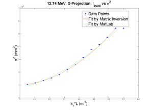
Gaussian fitted for part 1 of the image

Fitted Gaussian for part 1 of the image

       xl = 362;% center at 382
       xr = 404;
       yl = 241;% center at 271
       yr = 301;
xl: x left, xr: x right. yl: y left, yr: y right.

x-projection:

emit=0.322 +- 0.001 mm*mrad, emit_norm=8.022 +- 0.033 mm*mrad

beta=3.110 +- 0.003, alpha=0.906 +-0.002

HRRL 03-18-2011 Data Analysis Preliminary Results Gauss Fitted Part 1 Image.png


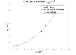
Gaussian fitted for part 2 of the image

Fitted Gaussian for part 2 of the image

       xl = 342;% center at 382
       xr = 424;
       yl = 241;% center at 271
       yr = 301;

x-projection:

emit=0.360 +- 0.001 mm*mrad, emit_norm=8.970 +- 0.031 mm*mrad

beta=1.993 +- 0.001, alpha=0.672 +-0.001


HRRL 03-18-2011 Data Analysis Preliminary Results Gauss Fitted Part 2 Image.png


Gaussian fitted for part 3 of the image

Fitted Gaussian for part 3 of the image

       xl = 342;% center at 382
       xr = 424;
       yl = 221;% center at 271
       yr = 321;
       

x-projection:

emit=0.360 +- 0.001 mm*mrad, emit_norm=8.970 +- 0.031 mm*mrad

beta=1.993 +- 0.001, alpha=0.672 +-0.001


HRRL 03-18-2011 Data Analysis Preliminary Results Gauss Fitted Part 3 Image.png


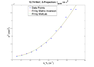
Gaussian fitted for part 4 of the image

Fitted Gaussian for part 4 of the image

       xl = 322;% center at 382
       xr = 444;
       yl = 221;% center at 271
       yr = 321;

x-projection:

emit=0.350 +- 0.001 mm*mrad, emit_norm=8.738 +- 0.032 mm*mrad

beta=1.344 +- 0.002, alpha=0.464 +-0.002

HRRL 03-18-2011 Data Analysis Preliminary Results Gauss Fitted Part 4 Image.png


Analysis with root

Q1_Scan, 42mA peak current, Scan Coil Current at positive 1.8_Amp

Image HRRL-03-18-2011-Analysis-with-root-Q1 Scan-42mA-peak-current-Scan-Coil-Current-at-positive-1.8 Amp-signal.png


Back grounds

HRRL-03-18-2011-Analysis-with-root-Q1 Scan-42mA-peak-current-Scan-Coil-Current-at-positive-1.8 Amp-bg-1.png HRRL-03-18-2011-Analysis-with-root-Q1 Scan-42mA-peak-current-Scan-Coil-Current-at-positive-1.8 Amp-bg-2.png HRRL-03-18-2011-Analysis-with-root-Q1 Scan-42mA-peak-current-Scan-Coil-Current-at-positive-1.8 Amp-bg-3.png HRRL-03-18-2011-Analysis-with-root-Q1 Scan-42mA-peak-current-Scan-Coil-Current-at-positive-1.8 Amp-bg-4.png HRRL-03-18-2011-Analysis-with-root-Q1 Scan-42mA-peak-current-Scan-Coil-Current-at-positive-1.8 Amp-bg-5.png HRRL-03-18-2011-Analysis-with-root-Q1 Scan-42mA-peak-current-Scan-Coil-Current-at-positive-1.8 Amp-bg-6.png HRRL-03-18-2011-Analysis-with-root-Q1 Scan-42mA-peak-current-Scan-Coil-Current-at-positive-1.8 Amp-bg-7.png HRRL-03-18-2011-Analysis-with-root-Q1 Scan-42mA-peak-current-Scan-Coil-Current-at-positive-1.8 Amp-bg-8.png HRRL-03-18-2011-Analysis-with-root-Q1 Scan-42mA-peak-current-Scan-Coil-Current-at-positive-1.8 Amp-bg-9.png HRRL-03-18-2011-Analysis-with-root-Q1 Scan-42mA-peak-current-Scan-Coil-Current-at-positive-1.8 Amp-bg-10.png


Signal Background
HRRL-03-18-2011-Analysis-with-root-Q1 Scan-42mA-peak-current-Scan-Coil-Current-at-positive-1.8 Amp-signal.png HRRL-03-18-2011-Analysis-with-root-Q1 Scan-42mA-peak-current-Scan-Coil-Current-at-positive-1.8 Amp-bg-1.png
These MATLAB fits are set to fit at 0.7 times above height of the peak.
Matlab fit to x profile Matlab fit to y profile
HRRL-03-18-2011-Analysis-with-root-Q1 Scan-42mA-peak-current-Scan-Coil-Current-at-positive-1.8 Amp-signal-Matlab Fit-x.png HRRL-03-18-2011-Analysis-with-root-Q1 Scan-42mA-peak-current-Scan-Coil-Current-at-positive-1.8 Amp-signal-Matlab Fit-y.png
sigma_x = 24.97 px sigma_y = 44.45 px
Blue: Signal, Red Background, Black: Subtraction HRRL-03-18-2011-Analysis-with-root-Q1 Scan-42mA-peak-current-Scan-Coil-Current-at-positive-1.8 Amp-signal bg sg-bg.png
signal HRRL-03-18-2011-Analysis-with-root-Q1 Scan-42mA-peak-current-Scan-Coil-Current-at-positive-1.8 Amp-surf-sg.png
background HRRL-03-18-2011-Analysis-with-root-Q1 Scan-42mA-peak-current-Scan-Coil-Current-at-positive-1.8 Amp-surf-bg.png
signal - background HRRL-03-18-2011-Analysis-with-root-Q1 Scan-42mA-peak-current-Scan-Coil-Current-at-positive-1.8 Amp-surf-sg-bg.png
signal HRRL-03-18-2011-Analysis-with-root-Q1 Scan-42mA-peak-current-Scan-Coil-Current-at-positive-1.8 Amp-contour-sg.png
background HRRL-03-18-2011-Analysis-with-root-Q1 Scan-42mA-peak-current-Scan-Coil-Current-at-positive-1.8 Amp-contour-bg.png
signal - background HRRL-03-18-2011-Analysis-with-root-Q1 Scan-42mA-peak-current-Scan-Coil-Current-at-positive-1.8 Amp-contour-sg-bg.png

Q6_Scan, 42mA peak current, Scan Coil Current at negative 2.5_Amp

Signal Background
HRRL-03-18-2011-Analysis-with-root-Q6 Scan-42mA-peak-current-Scan-Coil-Current-at-negative-2.5 Amp-signal.png HRRL-03-18-2011-Analysis-with-root-Q6 Scan-42mA-peak-current-Scan-Coil-Current-at-negative-2.5 Amp-bg-1.png
Matlab fit to x profile Matlab fit to y profile
set to fit at 0.2 times above height of the peak. set to fit at 0.7 times above height of the peak.
HRRL-03-18-2011-Analysis-with-root-Q6 Scan-42mA-peak-current-Scan-Coil-Current-at-negative-2.5 Amp-signal-Matlab Fit-x.png HRRL-03-18-2011-Analysis-with-root-Q6 Scan-42mA-peak-current-Scan-Coil-Current-at-negative-2.5 Amp-signal-Matlab Fit-y.png
sigma_x = 31.37 px sigma_y = 18.63 px

Lorentzian Fitting

Basic MATLAB Codes to fit Lorentzian:

File:Trial my Lorentzian fit.txt

File:Desum.txt

My MATLAB Fit code for beam

File:My Lorentzian fit.txt

File:Desum.txt

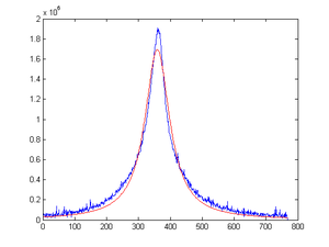
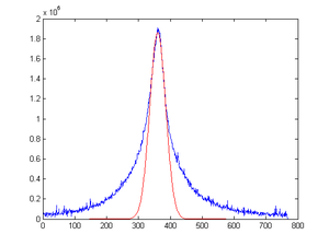
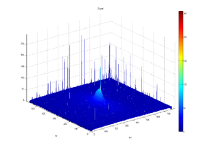
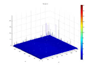
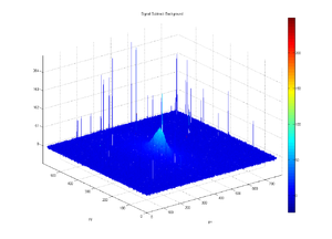
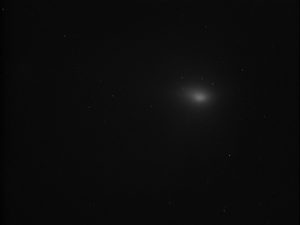
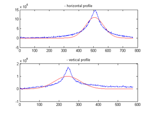
Here is an example fitting:

Signal Background fit
HRRL 03-18-2011 Lorentzian Fitting Example sg.png HRRL 03-18-2011 Lorentzian Fitting Example bg.png HRRL 03-18-2011 Lorentzian Fitting Example 1.png
height of the peak location of the peak half-width at half-maximum (HWHM)
1.6935e+006 358.9910 45.4280


Super Gaussian Fitting

Beam_Distribution_Beyond_RMS: File:Beam Distribution Beyond RMS.pdf

Basic MATLAB Codes to fit Super Gaussian:

File:Trial my Super Gaussian fit.txt

File:SupGau desum.txt

My MATLAB Fit code for beam

File:My Super Gaussian fit.txt

File:SupGau desum.txt

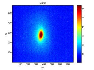
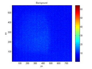
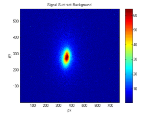
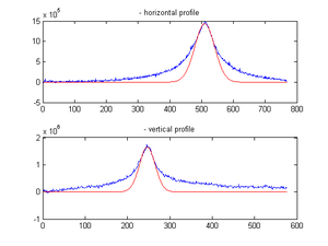
Here is an example fitting:

Signal Background fit
HRRL 03-18-2011 Lorentzian Fitting Example sg.png HRRL 03-18-2011 Lorentzian Fitting Example bg.png HRRL 03-18-2011 SupGau Fitting Example 1.png
height of the peak location of the peak base
8.0480e+003 359.6730 201.9112
sigma_0 N sigma
20.9204 0.8494 38.5672


HRRL_Emittance_Measurements_March14-18-2011