Difference between revisions of "TF ErrAna InClassLab"
(→Lab 11) |
|||
| (26 intermediate revisions by the same user not shown) | |||
| Line 53: | Line 53: | ||
What is binning? | What is binning? | ||
| − | The term binning is used to | + | The term binning is used to describe the process of grouping your data to determine how often (frequent) similar measurements occur. A bin represents the distance between two intervals in a histogram over which you are counting all measurements as the same value. |
For example: If I have the following data | For example: If I have the following data | ||
| Line 59: | Line 59: | ||
1.2, 1.6, 1.4, 1.8, 1.3 | 1.2, 1.6, 1.4, 1.8, 1.3 | ||
| − | and I create a histogram from 1-2 using only one bin, then I will have | + | and I create a histogram from 1-2 using only one bin, then I will have 5 counts showing in my histogram between 1 and 2 units. If however, I create 2 bins between 1 and 2 then I will have 3 counts in the bin corresponding to 1-1.5 and 2 counts in the 1.5-2.0 bin. |
You need to decide how to quantize the information to be presented in the histogram. One thing to consider is the systematic uncertainty of your device. If your device measures the temperature and has scale increments of 1/10 of a degree, you don't want to bin your temperature measurement using bin widths that are 1/10 or smaller. | You need to decide how to quantize the information to be presented in the histogram. One thing to consider is the systematic uncertainty of your device. If your device measures the temperature and has scale increments of 1/10 of a degree, you don't want to bin your temperature measurement using bin widths that are 1/10 or smaller. | ||
| Line 65: | Line 65: | ||
===Step 3: Filling the Histogram=== | ===Step 3: Filling the Histogram=== | ||
| − | The bins in a histogram are filled by rounding off the data according to the bin width. What happens if you are on the edge of a bin? Just follow the roundoff procedure | + | The bins in a histogram are filled by rounding off the data according to the bin width. What happens if you are on the edge of a bin? Just follow the roundoff procedure at [[Forest_Error_Analysis_for_the_Physical_Sciences#Round_Off]]. |
===Step 4: Labels=== | ===Step 4: Labels=== | ||
| Line 138: | Line 138: | ||
<pre> | <pre> | ||
| − | MyProgram() | + | void MyProgram() |
{ | { | ||
new TBrowser(); | new TBrowser(); | ||
| Line 182: | Line 182: | ||
<pre> | <pre> | ||
| − | MyProgram() | + | void MyProgram() |
{ | { | ||
TH1F *Hist1=new TH1F("Hist1","Hist1",50,-0.5,49.5); | TH1F *Hist1=new TH1F("Hist1","Hist1",50,-0.5,49.5); | ||
| Line 224: | Line 224: | ||
Create a histogram for the dice data from step 2.1. | Create a histogram for the dice data from step 2.1. | ||
| − | = | + | =Lab 3= |
== Uniform Distribution== | == Uniform Distribution== | ||
| Line 237: | Line 237: | ||
<pre> | <pre> | ||
| − | Udist() | + | void Udist() |
{ | { | ||
Int_t a=0; | Int_t a=0; | ||
| Line 296: | Line 296: | ||
</pre> | </pre> | ||
| − | = | + | =Lab 4= |
==Passing Arguments== | ==Passing Arguments== | ||
| Line 332: | Line 332: | ||
<pre> | <pre> | ||
| − | void PDF_Plot(Int_t N, double | + | void PDF_Plot(Int_t N, double Probability, Int_t NumTrials) |
{ | { | ||
TH1F *B30=new TH1F("B30","B30",100,0,100); | TH1F *B30=new TH1F("B30","B30",100,0,100); | ||
| − | + | for(Int_t i=0;i<N;i++) | |
| − | |||
| − | |||
{ | { | ||
| − | x=ROOT::Math::binomial_pdf(i, | + | double x=ROOT::Math::binomial_pdf(i,Probability,NumTrials); |
B30->Fill(i,x); | B30->Fill(i,x); | ||
} | } | ||
| Line 363: | Line 361: | ||
The goal of this lab is to overlay 2 distributions on top of each other | The goal of this lab is to overlay 2 distributions on top of each other | ||
| − | The functions below may be used to plot a binomial and poisson | + | The functions below may be used to plot a binomial and poisson distribution |
<pre> | <pre> | ||
| Line 482: | Line 480: | ||
for(Int_t i=0;i<100;i++) | for(Int_t i=0;i<100;i++) | ||
{ | { | ||
| − | x=ROOT::Math::binomial_pdf(i,p, | + | x=ROOT::Math::binomial_pdf(i,p,Max); |
Binomial->Fill(i,x); | Binomial->Fill(i,x); | ||
//printf("Step \t %d \n",i); | //printf("Step \t %d \n",i); | ||
| Line 511: | Line 509: | ||
;Note | ;Note | ||
| − | :<math>\sigma = \sqrt{\frac{N}{4}}</math> for Binomial | + | :<math>\sigma = \sqrt{Npq}= \sqrt{\frac{N}{4}}</math> for Binomial when p = q = 0.5 |
:<math>\sigma = \sqrt{\mu}</math> for Poisson | :<math>\sigma = \sqrt{\mu}</math> for Poisson | ||
| Line 646: | Line 644: | ||
All of the below | All of the below | ||
<pre> | <pre> | ||
| − | double landau_pdf(double x, double MostProbableValue, double sigma | + | double landau_pdf(double x, double MostProbableValue, double sigma ) |
double gamma_pdf(double x, double alpha, double theta, double x0 = 50) | double gamma_pdf(double x, double alpha, double theta, double x0 = 50) | ||
double gaussian_pdf(double x, double sigma = 1, double mean = 50) | double gaussian_pdf(double x, double sigma = 1, double mean = 50) | ||
| Line 749: | Line 747: | ||
:<math>C = A + \frac{B}{r^2}</math> | :<math>C = A + \frac{B}{r^2}</math> | ||
| − | Show that A = (12 <math>\pm</math> .76) <math>\times 10^1</math> and B = (31 <math>\pm</math> 0 | + | Show that A = (12 <math>\pm</math> .76) <math>\times 10^1</math> and B = (31 <math>\pm</math> 1.0 <math>\times 10^8</math>) Counts <math>\mbox{cm}^2</math> |
[[File:Forest_ErrAna_Lab_11_plot.png | 200 px]] | [[File:Forest_ErrAna_Lab_11_plot.png | 200 px]] | ||
| Line 788: | Line 786: | ||
[[Media:InvMat.C]] | [[Media:InvMat.C]] | ||
| + | |||
| + | |||
| + | <pre> | ||
| + | #ifndef __CINT__ | ||
| + | #include "TMatrixD.h" | ||
| + | #endif | ||
| + | |||
| + | |||
| + | void InvMat() | ||
| + | { | ||
| + | #ifdef __CINT__ | ||
| + | gSystem->Load("libMatrix"); | ||
| + | #endif | ||
| + | |||
| + | const Int_t nRowsCols = 2; | ||
| + | |||
| + | |||
| + | TMatrixD YLin(nRowsCols,nRowsCols); | ||
| + | YLin(0,0)=2.0; | ||
| + | YLin(0,1)=-1.0; | ||
| + | YLin(1,0)=-1.0; | ||
| + | YLin(1,1)=2.0; | ||
| + | |||
| + | YLin.Print(); | ||
| + | |||
| + | Float_t YlineDet; | ||
| + | YlineDet=YLin.Determinant(); | ||
| + | cout << "Determinant=" << YlineDet << endl; | ||
| + | |||
| + | TMatrixD YLinInvert(nRowsCols,nRowsCols); | ||
| + | YLinInvert=YLin.Invert(); | ||
| + | YLinInvert.Print(); | ||
| + | } | ||
| + | </pre> | ||
Check that you see the following output | Check that you see the following output | ||
| Line 891: | Line 923: | ||
|2 ||43.47||19 || ? | |2 ||43.47||19 || ? | ||
|- | |- | ||
| − | |3 || 26.56 || 18 || | + | |3 || 26.56 || 18 || 0.0876 |
|- | |- | ||
|4 || 24.91||17 || ? | |4 || 24.91||17 || ? | ||
| Line 901: | Line 933: | ||
|Order ||<math> \chi^2_1</math> || <math>\chi^2_2</math> ||N-n-1 || F | |Order ||<math> \chi^2_1</math> || <math>\chi^2_2</math> ||N-n-1 || F | ||
|- | |- | ||
| − | |2-3 ||43.47||26.56 || | + | |2-3 ||43.47||26.56 || 18 || 1.55 |
|- | |- | ||
|3-4 || 26.56 || 24.91 || 17 || 1.007 | |3-4 || 26.56 || 24.91 || 17 || 1.007 | ||
| Line 907: | Line 939: | ||
|4-5 || 24.91 || 23.29|| 16 || 1.006 | |4-5 || 24.91 || 23.29|| 16 || 1.006 | ||
|- | |- | ||
| − | |5-6 || 23.29|| 19.16 ||15 || 1. | + | |5-6 || 23.29|| 19.16 ||15 || 1.14 |
|} | |} | ||
| Line 953: | Line 985: | ||
[[File:TF_ErrAna_Lab15.png | 200 px]] | [[File:TF_ErrAna_Lab15.png | 200 px]] | ||
| + | |||
| + | [[ErrAnalLab15_Fitter]] | ||
| + | |||
| + | Root 6.08 | ||
=Lab 16= | =Lab 16= | ||
Latest revision as of 22:57, 5 February 2020
Start ROOT and Draw Histogram
Step 1
In this first lab your goal will be to start root and draw a histogram.
If you are on a Windows machine start the ROOT interpreter by double clicking on the Desctop icon which looks like a tree and says ROOT underneath it. If you are on a Unix machine set the environmental variable ROOTSYS to point to the base subdirectory containing the ROOT files and start root with the command $ROOTSYS/bin/root. You can set the ROOTSYS environmental variable under the bash shell with the command
export ROOTSYS=path
where path identifies the location of the root base subdirectory. My ROOT base subdirectory is located at ~/src/ROOT/root so I would execute the following shell command
export ROOTSYS=~/src/ROOT/root
Step 2
Define a variable to contain the desired histogram
TH1F *Hist1=new TH1F("Hist1","Hist1",50,-0.5,49.5);
The above function "TH1F" has 5 parameters and is a member of the class TH1.
The first parameter, "Hist1", creates a name for the histogram. The second parameter gives the histogram a title. I usually set the name and title to the same variable name I use to store the histogram. This allows me to look up the variable name of the histogram when I double click on the histogram from the browser listing. The third parameter (50) is an integer which identifies the number of "bins" the histogram will use to store information. The Fourth parameter (-0.5) is a real number identifying the numerical value to be used for the lowest bin and the fifth parameter is the value for the highest bin.
Step 3
The class TH1 contains a function "Fill" which you can you to insert data into the histogram. In the above example the variable "Hist1" was defined in terms of the class TH1. To use the Fill function which is defined within the class TH1 and associated with the histogram named Hist1 you use the command
Hist1->Fill(10);
The above Fill function will increment the counter for the bin in Hist1 which is associated with the numerical value "10"
Step 4
The TH1 class also has a function to graphically display the created histogram. The function is executed with the command
Hist1->Draw();
You should now see a histogram on your computer screen if ROOT is able to create a graphics window.
Lab 2
Histogram by Hand
Our goal is to construct a Histogram by hand (without using a computer).
Step 1: Range
The first step to creating a histogram is to determine what are the min and max values
Step 2: Binning
What is binning?
The term binning is used to describe the process of grouping your data to determine how often (frequent) similar measurements occur. A bin represents the distance between two intervals in a histogram over which you are counting all measurements as the same value.
For example: If I have the following data
1.2, 1.6, 1.4, 1.8, 1.3
and I create a histogram from 1-2 using only one bin, then I will have 5 counts showing in my histogram between 1 and 2 units. If however, I create 2 bins between 1 and 2 then I will have 3 counts in the bin corresponding to 1-1.5 and 2 counts in the 1.5-2.0 bin.
You need to decide how to quantize the information to be presented in the histogram. One thing to consider is the systematic uncertainty of your device. If your device measures the temperature and has scale increments of 1/10 of a degree, you don't want to bin your temperature measurement using bin widths that are 1/10 or smaller.
Step 3: Filling the Histogram
The bins in a histogram are filled by rounding off the data according to the bin width. What happens if you are on the edge of a bin? Just follow the roundoff procedure at Forest_Error_Analysis_for_the_Physical_Sciences#Round_Off.
Step 4: Labels
Properly label the abscissca and ordinate axis with names and UNITs.
Data for histogram
Create a histogram by hand using the following data.
Two dice are rolled 20 times. Create a histogram to represent the 20 trials below
| Trial | Value |
| 1 | 8 |
| 2 | 10 |
| 3 | 9 |
| 4 | 5 |
| 5 | 9 |
| 6 | 6 |
| 7 | 5 |
| 8 | 6 |
| 9 | 3 |
| 10 | 9 |
| 11 | 8 |
| 12 | 5 |
| 13 | 8 |
| 14 | 10 |
| 15 | 8 |
| 16 | 11 |
| 17 | 12 |
| 18 | 6 |
| 19 | 7 |
| 20 | 8 |
Create ROOT script to make Histogram
We are going to repeat Lab 1 but this time we will make a script to do the typing for us.
Step 1: Create Text file
Use an editor to create a text file.
In windows this could be the program "notepad" under the utilities menu (ie : Start->All Programs->Accessories->Notepad)
The important point is that you want to create and ASCII text file.
As a test, write the following in the text file
void MyProgram()
{
new TBrowser();
}
Now save the file as "test.C" in the root sub directory.
In Windows the root program launches such that it is within the subdirectory "C:\root". You should save your text file under the subdirectory "Local Disk (C:) root" using the "save as" menu.
If you did things correctly you can use the command completion function on the ROOT command line to load in your program
If you type the partial name
.L te
then hit the tab key, ROOT will complete the command or offer a list of commands you can use.
root[1] .L test
test/
test.C
If you are having trouble then just type the following within root
.L test.C
MyProgram();
You should see the ROOT browser open in a new window.
Step 2: Create a Program to fill histogram
Now let's create a program to create and fill a histogram like we did in Lab 1.
Using Notepad, or another editor, create and ASCII file with the following contents
void MyProgram()
{
  TH1F *Hist1=new TH1F("Hist1","Hist1",50,-0.5,49.5);
  Hist1->Fill(10);
  Hist1->Draw();
}
Save the file under the name "MyProgram.C"
Now launch root and type into the interpreter window
.x MyProgram.C
alternatively you can type
.L MyProgram.C
and then
MyProgram();
The above represents two different ways to do the same thing. One advantage of the
.L MyProgram.C
sequence is that you can get your program debugged by the C interpreter before you run it. When you are creating or editing a program you can reload the program into the interpreter after saving changes to a file to see it "compiles". So if you create a program that doesn't compile as expected you debug it, save the changes, reload it into the interpreter.
Dice Histogram
Create a histogram for the dice data from step 2.1.
Lab 3
Uniform Distribution
Our goal is to use ROOT to create a histogram representing a Uniform probability distribution.
ROOT has the following function defined
ROOT::Math::uniform_pdf(x,a,b,xo)
The above function returns the probability of observing the value for a uniform probability distribution spanning from to .
void Udist()
{
  Int_t a=0;
  Int_t b=10;
  TH2F *Udist=new TH2F("Udist","Udist",10,a,b,10,0,1);
  Udist->SetMarkerStyle(20); // sets the marker to a solid circle
  double x;
  x=ROOT::Math::uniform_pdf(1,0,10,0);
  Udist->Fill(1,x);
  x=ROOT::Math::uniform_pdf(2,0,10,0);
  Udist->Fill(2,x);
  x=ROOT::Math::uniform_pdf(3,0,10,0);
  Udist->Fill(3,x);
  x=ROOT::Math::uniform_pdf(4,0,10,0);
  Udist->Fill(4,x);
  x=ROOT::Math::uniform_pdf(5,0,10,0);
  Udist->Fill(5,x);
  x=ROOT::Math::uniform_pdf(6,0,10,0);
  Udist->Fill(6,x);
  x=ROOT::Math::uniform_pdf(7,0,10,0);
  Udist->Fill(7,x);
  x=ROOT::Math::uniform_pdf(8,0,10,0);
  Udist->Fill(8,x);
  x=ROOT::Math::uniform_pdf(9,0,10,0);
  Udist->Fill(9,x);

  //Grades->Sumw2();
  Udist->Draw("P");
}
ROOT GUI practice
During the lab the instructor will demonstrate how to make changes to Histograms using the ROOT GUI.
Histogram Font labels
Readability is a key ingredient to producing histograms that is often neglected. You will be shown how to increase font sizes and change font types to produce a more readable histogram that is of publication quality.
Histogram module
Here you will be shown how to change markers and other attributes of the histogram.
Rebinning
Changing bin sizes can allow you to change the statistical precision of a measurement at the cost of resolution.
Uniform dist Program
Now see if you can convert the program above which drew a uniform distribution histogram to a program which can do the same thing for arbitrary values of a & b.
hint:
Udist(Int_t N,Int_t a,Int_t b)
Lab 4
Passing Arguments
Write a function for the ROOT interpreter which accepts three arguments, N, mean, variance. where N= number of counts
void PDF_Plot(Int_t N, double Mean, double Variance)
{

  printf("PDF plotting %d event with mean %g and variance %g\n",N,Mean,Variance);

}
for loops
Now add a loop which repeats N times
void PDF_Plot(Int_t N, double Mean, double Variance)
{

  printf("PDF plotting %d event with mean %g and variance %g\n",N,Mean,Variance);

  for(Int_t i=0;i<N;i++)
    printf("Step \t %d \n",i);
}
Binomial Distribution plot
Now we will do a weighted 1-D histogram. This type of histogram allows you to have non integer counts. This will allow us to plot functions without binning the "y" axis like we did in the previous lab.
 void PDF_Plot(Int_t N, double Probability, Int_t NumTrials)
{
  TH1F *B30=new TH1F("B30","B30",100,0,100);


   for(Int_t i=0;i<N;i++)
    {
      double x=ROOT::Math::binomial_pdf(i,Probability,NumTrials);
      B30->Fill(i,x);
    }
 B30->Draw();

}
You execute the above program using the ROOT commands
root [0] .L PDF_Plotr.C
root [1] PDF_Plot(100,0.5,60)
Uniform Dist
Now can you go back to Lab_3 and plot the Uniform distribution using a 1-D histogram?
Lab 5
The goal of this lab is to overlay 2 distributions on top of each other
The functions below may be used to plot a binomial and poisson distribution
TH1F *B30=new TH1F("B30","B30",100,0,100);
TH1F *P30=new TH1F("P30","P30",100,0,100);

void Binom_Plot(Int_t k, double p, Int_t n)
{

  // k= number of successful trials
  //p = probability of success
  //N= number of trials
  // Example: the number of heads = k after flipping a coin n times, p=0.5

  printf("PDF plotting %d event with prob %g and  %d trials\n",k,p,n);

  for(Int_t i=0;i<k;i++)
    {
            x=ROOT::Math::binomial_pdf(i,p,n);
            B30->Fill(i,x);
      //printf("Step \t %d \n",i);
 }
   B30->Draw();

}
void Pois_Plot(Int_t Nmin, Int_t Nmax, double Mean)
{

  // N = # of events in time interval t
  // mean = probability per unit interval * interval

  printf("PDF plotting %d event with mean %g \n",Nmin,Mean);

  //  for(Int_t i=Nmin;i<Nmax;i++)
  for(Int_t i=Nmin;i<Nmax;i++)
    {
            x=ROOT::Math::poisson_pdf(i,Mean);
            P30->Fill(i,x);
            //      printf("Step \t %d \t %g\n",i,x);
 }
   P30->Draw();

}
create Binomial Distribution
Binom_Plot(100,0.166667,10)
create a Poisson Distribution
Pois_Plot(0, 100, 1.667);
overlay them
B30->Draw();
P30->Draw("same");
Your goal in this lab will be to understand all of the above and plot both distributions above using the same mean for each but a different mean than the one used above. You will also customize the plot with colors, dashed lines, and titles to more easily distinguish the two distributions.
Lab 6
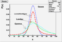
The goal in this lab is to compare the Binomial, Poisson, and Gaussian distributions. Repeat step Lab 5 and include a Gaussian distribution.
The difference will be to perform the above plots with a large average from 10 -70. Try to guess a Gaussian which will overlap with the Binomial and Poisson distributions.
The function below may be useful
ROOT::Math::gaussian_pdf(x,5.477,30)
mean = 30, sigma = 5.477
Helpful ROOT commands
 TH1F *Poisson=new TH1F("Poisson","Poisson",100,0,100);
  Poisson->SetLineColor(3);
  Poisson->SetLineWidth(3);
  Poisson->SetLineStyle(4);
If you give up try the program below
void BPG_Plot(Int_t Min, Int_t Max, double p)
{
  // k= number of successful trials
  //p = probability of success
  //N= number of trials
  // Example: the number of heads = k after flipping a coin n times, p=0.5
  TH1F *Binomial=new TH1F("Binomial","Binomial",100,0,100);

  Binomial->GetXaxis()->SetTitle("x");
  Binomial->GetXaxis()->SetTitleSize(0.06);
  Binomial->GetXaxis()->CenterTitle();
  Binomial->GetYaxis()->SetTitle("P(x)");
  Binomial->GetYaxis()->SetTitleOffset(1.2);
  Binomial->GetYaxis()->SetTitleSize(0.06);
  Binomial->SetLineColor(4);
  Binomial->SetLineWidth(3);
  Binomial->SetLineStyle(2);

  TH1F *Poisson=new TH1F("Poisson","Poisson",100,0,100);
  Poisson->SetLineColor(3);
  Poisson->SetLineWidth(3);
  Poisson->SetLineStyle(4);
 TH1F *Gauss=new TH1F("Gauss","Gauss",100,0,100);

 Gauss->SetLineColor(2);
  Gauss->SetLineWidth(3);
  Gauss->SetLineStyle(9);
  double Mean, sigma;
  for(Int_t i=0;i<100;i++)
    {
      x=ROOT::Math::binomial_pdf(i,p,Max);
      Binomial->Fill(i,x);
      //printf("Step \t %d \n",i);
            Mean=p*(Max-Min);
            x=ROOT::Math::poisson_pdf(i,Mean);
            Poisson->Fill(i,x);
            sigma=sqrt(Mean);
            x=ROOT::Math::gaussian_pdf(i,sigma,Mean);
            Gauss->Fill(i,x);

 }
   Binomial->Draw();
   Poisson->Draw("same");
   Gauss->Draw("same");


}
Lab 7
The goal in this lab is to compare the Binomial, Poisson, and Gaussian distributions by taking the difference between the two distributions.
Construct 2 graphs representing how well the Gaussian distribution approximates the Binomial and Poisson distributions at limits where such approximations are valid.
- Note
- for Binomial when p = q = 0.5
- for Poisson
A function appears in lab 6 above which overlays the three distributions. Feel free to start with that function, or write your own, to plot the difference between a Binomial and gaussian distribution. Consider plotting the difference squared after you realize that the differences average out to a value close to zero.
I used the functions below to draw the difference plots and xmgrace to draw the Difference -vs- N plot.
Lab 8
The table below contains information on the measurement of the length of a block and the number of times the same value was observed.
| Lenght (cm) | # of observations |
| 18.9 | 1 |
| 19.0 | 0 |
| 19.1 | 1 |
| 19.2 | 2 |
| 19.3 | 1 |
| 19.4 | 4 |
| 19.5 | 3 |
| 19.6 | 9 |
| 19.7 | 8 |
| 19.8 | 11 |
| 19.9 | 9 |
| 20.0 | 5 |
| 20.1 | 7 |
| 20.2 | 8 |
| 20.3 | 9 |
| 20.4 | 6 |
| 20.5 | 3 |
| 20.6 | 2 |
| 20.7 | 2 |
| 20.8 | 2 |
| 20.9 | 2 |
| 21.0 | 4 |
| 21.1 | 0 |
| 21.2 | 1 |
The assumption is that the parent population is a Gaussian with a mean cm and cm.
Below is a program and a data file which you can use to create a histogram of the data in the above table.
You must save the data file as filename "length.dat" for now
1.) Run the program and create a histogram.
2.)Open the Draw Panel and choose the option "SIMPLE" Error
3.) What has ROOT used to estimate the statistical error? (, , 1/N , ...)
4.) Assuming the parent distribution has cm and cm, use the Gaussian CDF functions
- ROOT::Math::normal_cdf(19.0,0.5,20) Probability that you measure a value less than or equal to (lower tail)
or
- ROOT::Math::normal_cdf_c(21.0,0.5,20) Probability that you measure a value greater than or equal to (upper tail)
to determine the probability you should get data less than 19 cm and greater than 21 cm.
also try
ROOT::Math::normal_cdf(18.9,0.5,20)
and
ROOT::Math::normal_cdf_c(21.2,0.5,20)
5.) Now determine how many events you should see outside of 2 ( 1 ) .
Send me an e-mail describing your results for parts 3, 4 & 5 above.
If time permits:
6.) Now edit the program so a Histogram is created with the Parent Gaussian distribution having a and cm .
Lab 9
In this lab you will illustrate the following PDF distributions
One of the below
double	breitwigner_pdf(double x, double gamma, double x0 = 50)
double	cauchy_pdf(double x, double b = 1, double x0 = 0)
All of the below
double	landau_pdf(double x, double MostProbableValue, double sigma )
double	gamma_pdf(double x, double alpha, double theta, double x0 = 50)
double	gaussian_pdf(double x, double sigma = 1, double mean = 50)
Start by overlaying them on the same graph and pointing out differences.
Compare Skewness and Kurtosis.
Create a table of Mean, Skewness, and Kurtosis for each distributions using the same x_0 such that they are similar.
Try plotting the functions below individually.
double beta_pdf (double x, double a, double b)
double exponential_pdf(double x, double lambda, double x0 = 0)
Lab 10
A metal rod is placed with its ends in two different temperature baths. One bath is at zero degree Celsius and the other at 100. The temperature along the rod is measure and given in the table below.
| Trial | Position (cm) | Temperature (Celsius) |
| 1 | 1.0 | 15.6 |
| 2 | 2.0 | 17.5 |
| 3 | 3.0 | 36.6 |
| 4 | 4.0 | 43.8 |
| 5 | 5.0 | 58.2 |
| 6 | 6.0 | 61.6 |
| 7 | 7.0 | 64.2 |
| 8 | 8.0 | 70.4 |
| 9 | 9.0 | 98.8 |
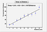
Fit the above data assuming a linear function
T = A + b X
Using the following program
Media:Forest_ErrAna_LinFit1.C File:Forest ErrAna LinFit1.C
Now alter the program to determine the error in the parameters
Try to produce a plot which looks better than this
Lab 11
Radiation attenuation as a function of distance from the source.
A student uses a Geiger Muller tube to measure the count rate as a function of distance. The detector is placed at several distances away from the source and the count rate is measured over several time intervals to get a measure of the uncertainty in each measurement. The table below lists the results.
| Trial | Distance (m) | Counts | Count Err [sqrt(N)] |
| 1 | 20 | 901 | 30.0 |
| 2 | 25 | 652 | 25.5 |
| 3 | 30 | 443 | 21.0 |
| 4 | 35 | 339 | 18.4 |
| 5 | 40 | 283 | 16.8 |
| 6 | 45 | 281 | 16.8 |
| 7 | 50 | 240 | 15.5 |
| 8 | 60 | 220 | 14.8 |
| 9 | 75 | 180 | 13.4 |
| 10 | 100 | 154 | 12.4 |
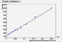
Perform a linear fit using the above data for the functional dependence of
Show that A = (12 .76) and B = (31 1.0 ) Counts
Lab 12
The Correlation Coefficient is defined as
Insert the above formula into the UNWEIGHTED fit for Lab 10 and calculate R.
The probability that the data are NOT CORRELATED is given by
- Both functions within ROOT below return the same value
 ROOT::Math::tgamma(Double_t x)
 TMath::Gamma(Double_t x)
Use the above formula to calculate the probability that the data are not correlated.
Lab 13
Matrix inversion
Run the program below to invert the matrix:
#ifndef __CINT__
#include "TMatrixD.h"
#endif


void InvMat()
{
#ifdef __CINT__
  gSystem->Load("libMatrix");
#endif

  const Int_t nRowsCols  = 2;


  TMatrixD YLin(nRowsCols,nRowsCols);
  YLin(0,0)=2.0;
  YLin(0,1)=-1.0;
  YLin(1,0)=-1.0;
  YLin(1,1)=2.0;

  YLin.Print();

  Float_t YlineDet;
  YlineDet=YLin.Determinant();
  cout << "Determinant=" <<  YlineDet << endl;

  TMatrixD YLinInvert(nRowsCols,nRowsCols);
  YLinInvert=YLin.Invert();
  YLinInvert.Print();
}
Check that you see the following output
root [0] .L InvMat.C
root [1] InvMat()

2x2 matrix is as follows

     |      0    |      1    |
-------------------------------
   0 |          2          -1
   1 |         -1           2

Determinant=3

2x2 matrix is as follows

     |      0    |      1    |
-------------------------------
   0 |     0.6667      0.3333
   1 |     0.3333      0.6667
Now invert the following matrix.
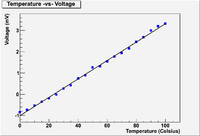
Linear Fit to Temp -vs- Voltage data
A thermocouple is calibrated by measuring the temperature of the thermocouple as a function of the output voltage of a circuit which uses the thermocouple as a resister. The measurements are given below.
Temp   Volts
(C)       (mV)
0.      -0.849
20.     -0.196
40.     0.734
60.     1.541
80.     2.456
100.    3.318
Determine the parameters and for a linear fit
ie:
using both the Method of Determinants and Linear Regression (Matrix inversion)
- Assume the uncertainty in V is 0.05 mV.
2nd order Poly Fit to Temp-vs- Voltage data
Perform a 2nd order polynomial fit (with uncertainties) the to Temp -vs- Voltage data in the previous subsection.
ie:
Lab 14
Determine the following for a nth order fit, where 2 < n < 4, to the expanded data in lab 13 given below .
Temp, Voltage
(Celsius), (mV)
0.      -0.849
5.0     -0.738
10.     -0.537
15.     -0.354
20.     -0.196
25.     -0.019
30.     0.262
35.     0.413
40.     0.734
45.     0.882
50.     1.258
55.     1.305
60.     1.541
65.     1.768
70.     1.935
75.     2.147
80.     2.456
85.     2.676
90.     2.994
95.     3.200
100.    3.318
P-Value
| Order | p-value | ||
| 2 | 43.47 | 19 | ? |
| 3 | 26.56 | 18 | 0.0876 |
| 4 | 24.91 | 17 | ? |
F-test
| Order | N-n-1 | F | ||
| 2-3 | 43.47 | 26.56 | 18 | 1.55 |
| 3-4 | 26.56 | 24.91 | 17 | 1.007 |
| 4-5 | 24.91 | 23.29 | 16 | 1.006 |
| 5-6 | 23.29 | 19.16 | 15 | 1.14 |
root [0]  ROOT::Math::fdistribution_pdf(1.55,19,18,0)
(double)3.52060154633677236e-01
- Interpretation
- An Ftest of the Chisqrd ratio between a 2nd and 3rd order was .35 (35%).
root [1]  ROOT::Math::fdistribution_pdf(1.007,18,17,0)
(double)8.16466777630106444e-01
- Interpretation
- Redoing the Ftest comparing 3 and 4th order resulted in 0.82 (82%) compared to 33% for the 3rd order fit.
root [8]  ROOT::Math::fdistribution_pdf(1.006,16,17,0)
(double)7.92881516441281908e-01
- Interpretation
- Redoing the Ftest comparing 4 and 5th order results in 0.79 (79%) compared to 82% for the 4th order fit.
root [14]  ROOT::Math::fdistribution_pdf(1.297,15,16,0)
(double)5.22426549278646291e-01
- Interpretation
- Redoing the Ftest comparing 5 and 6th order results in 0.52(52%) compared to 79% for the 5th order fit.
- Conclusion
- The fit does not substantially improve beyond using a 4th order polynomial.
Lab 15
Parameter space
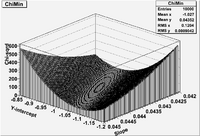
For the linear fit in Lab 14, construct a 2-D contour plot representing the value of for several different values of y-intercept and slope parameters.
Root 6.08
Lab 16
Our goal will be to adapt the C++ programs from Bevington's Chapt 8 to run within the ROOT framework and use it to fit the following data
File:Bev Chapt8 Time-vs-Counts.txt
to the function
But before we jump into fitting the above data, let's try to use the Grid search to fit the Linear data which produced the contour plot in Lab 15.
Grid Search
The following function to perform a Grid search is from Bevington
File:Bevington GridSearchFunction.C
ChiSqrdCalc
To implement the above function from Bevington you will need to calculate for a given set of parameters.
The following is one function you might consider using
Int_t NumPoints=0;
Float_t x[100],y[100],errory[100];
Double_t chiSq1,chiSq2,chiSq3;

//______________________________________________________________________________
Double_t func(float x,float y,Double_t *par)
{
  // Bevington Chapt 5 Fit function
  //  Double_t value=( par[0]+par[1]*exp((-1.0)*x/par[3])+par[2]*exp((-1.0)*x/par[4]));

  //Temp-vs-Voltage Fit function

  Double_t value=( par[0]+par[1]*x);

 return value;
}

//______________________________________________________________________________
Double_t CalcChiSq(Int_t &npar, Double_t *par, Int_t iflag)
{
//calculate chisquare
   Double_t chisq = 0;
   Double_t delta;
   for (Int_t i=0;i<NumPoints; i++) {
     delta  = (y[i]-func(x[i],y[i],par))/errory[i];
     chisq += delta*delta;
   }
   return(chisq);
}
In the above function the data are stored in the global arrays x[i], y[i] and errory[i]. The number of parameters is passed to the function using the variable npar and the actual parameters, stored in an array, are passed using the variable par.
The variable NumPoints is also a global variable and determines how many data points are used to calculate .
void GridTest(void )
{
   const Int_t NPar=2;
   Double_t Parameter[NPar],ParameterStepSize[NPar];
   //   Parameter[0]=-1.00503;
   //   Parameter[1]=0.043144;
   Parameter[0]=-0.88;
   Parameter[1]=0.041;

   ParameterStepSize[0]=0.01;
   ParameterStepSize[1]=0.001;
   printf("Iinitial ChiSQR=%g\n",CalcChiSq(NPar, Parameter, 0));
   GridLS(NPar, Parameter, ParameterStepSize);
}
PlotResults
void PlotResults(Int_t npar, Double_t *Params)
{
   Float_t yfit[100];


  if(NumPoints==0)
    {
      printf("Data arrays are not filled\n execute function \n\tLoadDataArrays\n");
      return;
    }

   /*
   for(Int_t i=0;i<npar;i++)
     {
       printf("Params[%d]=%g\n",i,Params[i]);
     }
   */

   TGraph *gr = new TGraphErrors(NumPoints,x,y,0,errory);
   gr->SetTitle("Counts -vs- Time");
   gr->GetXaxis()->SetTitle("Time (s)");
   gr->GetYaxis()->SetTitle("Counts");
   gr->SetMarkerColor(4);
   gr->SetMarkerStyle(21);
   gr->Draw("AP");
   //   gr->Draw();
   //Fit results

   for(Int_t i=0;i<NumPoints;i++)
     {
       //       yfit[i]=func(x[i],y[i],Parameters);
       yfit[i]=func(x[i],y[i],Params);
       //       printf("x[%d]=%g\ty[%d]=%g\tyfit=%g\n",i,x[i],i,y[i],yfit[i]);
     }

      TGraph *grfit = new TGraph(NumPoints,x,yfit);
      grfit->Draw();

}

