Difference between revisions of "Simulating Particle Trajectories"
| (2 intermediate revisions by the same user not shown) | |||
| Line 3: | Line 3: | ||
'''Description of Problem''' | '''Description of Problem''' | ||
| − | + | Essentially what we need to do is determine the trajectory of charged particles in an electromagnetic field. In simple cases, such as when the fields are uniform, the appropriate set of dynamical equations can be solved analytically. However, for the "silver" permanent magnet we plan on using for the pair spectrometer, the fields are anything but uniform. In such a case, the system must be solved numerically. | |
| − | + | '''Description of PAIRSPEC Code''' | |
| − | |||
| − | |||
| − | |||
| − | |||
| − | |||
| − | |||
| − | |||
| − | '''Description of Code''' | ||
The code, [[New Particle Trajectory Code|found here]], solves the above system of equations using an embedded 8th order Runge-Kutta Prince-Dormand method with 9th order error estimates with adaptive stepsize control, as implemented in the GNU Scientific Library [http://www.gnu.org/software/gsl]. The files include the relevant source and a script which should build the executable on any unix system with GSL installed in the usual place. The program also requires the ncurses library (standard with just about any linux distribution), the PGPLOT graphics library [http://www.astro.caltech.edu/~tjp/pgplot/], and the RDYNLAB library [[RDYNLAB|found here]]. | The code, [[New Particle Trajectory Code|found here]], solves the above system of equations using an embedded 8th order Runge-Kutta Prince-Dormand method with 9th order error estimates with adaptive stepsize control, as implemented in the GNU Scientific Library [http://www.gnu.org/software/gsl]. The files include the relevant source and a script which should build the executable on any unix system with GSL installed in the usual place. The program also requires the ncurses library (standard with just about any linux distribution), the PGPLOT graphics library [http://www.astro.caltech.edu/~tjp/pgplot/], and the RDYNLAB library [[RDYNLAB|found here]]. | ||
| Line 67: | Line 59: | ||
For the "interactive mode", the input file is identical to the input file for "detailed mode", with the exception of the -1 on the first line. The trajectories are plotted to the screen, and a control dialog appears in the terminal, as shown in the screenshot below. Upon exiting, the program writes a "detailed mode" input file for the last adjustment to "pairspec.in". | For the "interactive mode", the input file is identical to the input file for "detailed mode", with the exception of the -1 on the first line. The trajectories are plotted to the screen, and a control dialog appears in the terminal, as shown in the screenshot below. Upon exiting, the program writes a "detailed mode" input file for the last adjustment to "pairspec.in". | ||
| − | [[Image:pairspec_screenshot.jpg| | + | [[Image:pairspec_screenshot.jpg|600px]] |
An older version of the code that did not include all of the features and had more limitations, and wrote different output flags can be found [[Particle Trajectory Code|here]]. | An older version of the code that did not include all of the features and had more limitations, and wrote different output flags can be found [[Particle Trajectory Code|here]]. | ||
Latest revision as of 17:56, 18 June 2009
This article discusses numerical simulations of particle trajectories in the "silver" permanent magnet.
Description of Problem
Essentially what we need to do is determine the trajectory of charged particles in an electromagnetic field. In simple cases, such as when the fields are uniform, the appropriate set of dynamical equations can be solved analytically. However, for the "silver" permanent magnet we plan on using for the pair spectrometer, the fields are anything but uniform. In such a case, the system must be solved numerically.
Description of PAIRSPEC Code
The code, found here, solves the above system of equations using an embedded 8th order Runge-Kutta Prince-Dormand method with 9th order error estimates with adaptive stepsize control, as implemented in the GNU Scientific Library [1]. The files include the relevant source and a script which should build the executable on any unix system with GSL installed in the usual place. The program also requires the ncurses library (standard with just about any linux distribution), the PGPLOT graphics library [2], and the RDYNLAB library found here.
When executing the code, you must specify an input file on the command line. The input file is fairly simple. The first line of the input file is either a "0" or some integer greater than zero, and tells the program to run in "detailed output" or "scan" mode, respectively. In the latest version of the code, an interactive mode is also available by putting a -1 on this first line.
In "detailed output" mode, the next five lines specify the energy of the initial gamma ray, the energy of the electron (the energy of the positron is assumed to be the difference of these two numbers), the angle between the axis of the magnet and the photon beam, the "Y" position of the conversion site above the magnet yoke, and the "X" position of the conversion site relative to the left edge of the magnet. In "scan" mode, the integer on the first line tells the program how many cases to run. Only two additional lines are needed: the energy of the photon and the "X" position of the conversion site. Examples of such input files are provided here (detailed mode) and here (scan mode).
The program output also depends on the program mode. In the "detailed output" mode, everything is written to stdout, and can be directed to a file using the ">" director. The output begins with a header, each line of which begins with the "#" character. The header lists the physical properties of the particle, the conditions read from the input file, and the corresponding initial positions and momenta of the electron and positron. Following the header, the program writes four columns of data: the time (in seconds) and the x, y, and z coordinates (in meters).
In "scan" mode, the program randomly selects an electron energy, angle of the magnet axis relative to the beam, and a conversion site "Y" coordinate, all subject to appropriate reasonable limits and kinematic constraints. It then models the trajectory of the particle until either the particle is sufficiently far from the detector, or a certain maximum time is reached. The program then evaluates the angles of the particles' final trajectories relative to the initial photon beam and assigns a flag as follows:
| 0 | Both particles have exit angles greater than 90 degrees (ideal) |
| 1 | Only the electron has an exit angle greater than 90 degrees |
| 2 | Only the positron has an exit angle greater than 90 degrees |
| 3 | Neither particle has an exit angle greater than 90 degrees, but both leave the magnet. |
| 4 | The electron hits the yoke |
| 5 | The positron hits the yoke |
| 6 | Both particles hit the yoke |
| 7 | The electron gets trapped in the field |
| 8 | The positron gets trapped in the field |
| 9 | Both particles get trapped in the field |
Ideally we want to tag both particles in coincidence with both particles exiting the beam at an angle greater than 90 degrees, hence the classifications in the table above.
Also, in "scan" mode, the program writes output to three places. The primary output is written to stdout, and can be directed to a file. This output consists of a header (each line of which begins with "#") listing the parameters passed to the program in the input file. The output itself is in five columns, consisting of the iteration number, the energy of the electron (in MeV), the angle of the magnet axis relative to the beam (in degrees), the height of the conversion site above the yoke (in meters), and the output flag as described above. Each line of output ends with a character "X" to facilitate extracting iterations that returned a particular flag using the grep command.
Progress output is written to stderr, and for each run that results in a flag greater than one an input file (for "detailed output" mode) is written.
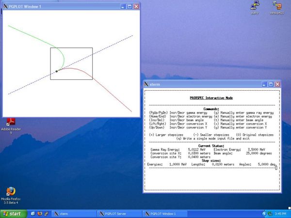
For the "interactive mode", the input file is identical to the input file for "detailed mode", with the exception of the -1 on the first line. The trajectories are plotted to the screen, and a control dialog appears in the terminal, as shown in the screenshot below. Upon exiting, the program writes a "detailed mode" input file for the last adjustment to "pairspec.in".
An older version of the code that did not include all of the features and had more limitations, and wrote different output flags can be found here.
The magnetic field, as implemented in the code
The measured magnetic field for the "silver" permanent magnet can be found here or here. To implement this field in the code, I performed a least squares fit to the data using a function of the form
with
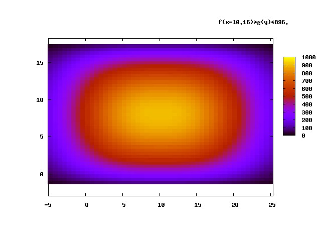
where and are in centimeters, is the maximum field (0.0896 Tesla), and the and are constants. These functional forms were chosen due to their good fit to the provided measured fields. The code explicitly puts a lower bound of zero on the magnetic field at any point in space. The constants turn out to be 1.0019, 0.064866, 2.74157, and 23.4233, and the constants are -0.0107702, 0.174007, and 0.305011. A map of this functional form for the field is shown below. The units for the field are in Gauss (they were converted to Tesla in the code), and the units for the x and y axes are centimeters. The lower left corner of the magnet is at (0,0).
Radiative Power Loss
The code accounts for power radiated away as the charged particles accelerate. Such power loss is given by the Lienard formula,
For energies and speeds typical of what we expect to see in the pair spectrometer, these power losses are negligible. The code includes such power losses through the RDYNLAB library.
Results of parameter space scans
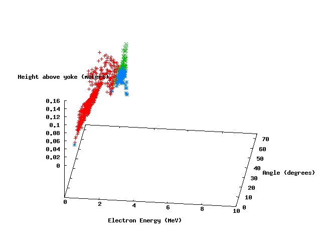
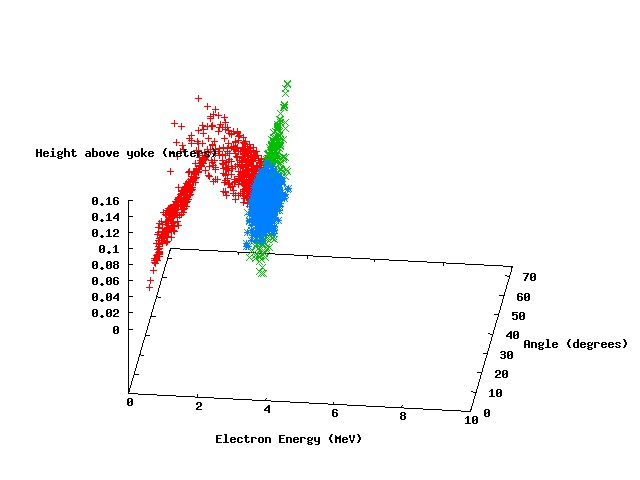
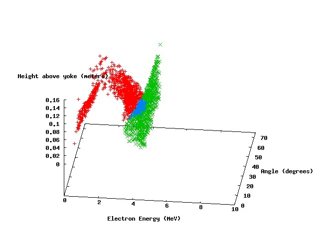
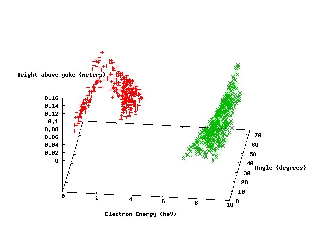
The following scatter plots show the results of four parameters scans, with photon energies of 3 MeV, 4 Mev, 5 MeV, and 10 MeV, respectively.
The points in red represent parameter sets where the electron leaves the magnetic field with an exit angle greater than 90 degrees. The green points represent a similar condition for the positron, and the blue points represent parameter sets where both particles leave with exit angles greater than 90 degrees (our "ideal" scenario). It can be seen that ideal parameter space exists for incident photon energies of 3, 4, and 5 MeV. There is a significant set of parameters at 5 MeV incident energy that meet the ideal criteria.
"Ideal" orientation of magnet for 5 MeV photons
The center of the ideal region of parameter space for 5 MeV photons has (approximately) the following characteristics:
- The electron energy is about 3.5 MeV (meaning the positron energy is about 1.5 MeV)
- The angle between the magnet axis and the original beam is about 50 degrees
- The conversion site is at the left edge of the magnet, about 2 centimeters above the yoke.
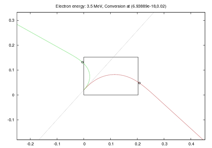
The figure below shows the trajectories of the electron (red) and the positron (green) for these parameters. The black box represents the magnet (with the return yoke at the bottom), and is roughly to scale. The dotted gray line represents the photon beam line.
One possible set of locations for the two detectors is to place one adjacent to the left edge of the magnet (left as seen in this graph) with the center at a distance of 0.132 meters above the yoke and displaced 0.005 cm from the left edge of the magnet. The other detector could have its center placed 0.005 meters from the right edge of the magnet and 0.048 meters above the return yoke. These suggested positions can be seen in the PDF document in the next section. Certainly, other positions would also work.
Pairs produced elsewhere on the beam
It is possible that the photons will pair produce in air at other locations on the beam, or that the electron produced will not carry 3.5 MeV of the total energy. This document shows the trajectories for the particles in these other scenarios. The electron energy and the "X" position of the conversion site are shown at the top of each graph. The black circles represent possible locations for the detectors. It appears that only the parameters described above will cause a coincidence in both detectors.
