Difference between revisions of "LB SageBrushWork PostDefense"
| (411 intermediate revisions by 2 users not shown) | |||
| Line 1: | Line 1: | ||
=Mass Information= | =Mass Information= | ||
| − | The target masses are as follows | + | Note that only 2 samples were produced using the oven method (0.04% and 10%). The target masses are as follows |
==50% Se/Sage Sample== | ==50% Se/Sage Sample== | ||
| Line 273: | Line 273: | ||
740-1020 (Mixture) | 740-1020 (Mixture) | ||
| + | |||
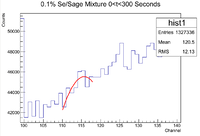
| + | The histogram representing the time cuts for the third run are shown below | ||
| + | |||
| + | It would appear that first two time cuts are difficult to determine because the Co-60 flag's counts are on the same order as the sample's, so watch out for this next time! Each run should be roughly 300 seconds for the sample and 60 seconds for the Co-60 flag, so check the histograms to make sure there are no Co-60 lines to correct for this. To double check these time cuts I looked for Cl-34m in the mixture (which according to my 10% analysis was not present in the pure Se sample) and the Co-60 lines that may have overlapped. It seems there is a line near 1773 keV present in the mixture, but the 1332 keV line is missing in the mixture. Keep an eye out. | ||
| + | |||
| + | [[File:0 04Percent SeSage TimeCuts 1DHistogram Run3.png|200px]] | ||
| + | |||
| + | 0-300 (Mixture,145 keV 1173 present | 1332 keV not present,good) | ||
| + | |||
| + | 305-350 (Co-60, good) | ||
| + | |||
| + | 360-650 (Pure Se, good) | ||
| + | |||
| + | 660-710 (Co-60, good) | ||
| + | |||
| + | 720-940 (Mixture, good) | ||
| + | |||
| + | 1020-1070 (Co-60, good) | ||
| + | |||
| + | 1100-1240 (Pure Se, good) | ||
| + | |||
| + | 1270-1310 (Co-60, good) | ||
| + | |||
| + | 1320-1630 (Mixture, good) | ||
| + | |||
| + | 1660-1720 (Co-60, good) | ||
| + | |||
| + | 1740-2030 (Pure Se, good) | ||
| + | |||
| + | 2040-2120 (Co-60, good) | ||
| + | |||
| + | 2130-2420 (Mixture, good) | ||
| + | |||
| + | 2430-2490 (Co-60, good) | ||
| + | |||
| + | 2500-2800 (Pure Se, good) | ||
| + | |||
| + | 2810-2850 (Co-60, good) | ||
| + | |||
| + | 2880-3150 (Mixture, good) | ||
| + | |||
| + | 3170-3220 (Co-60, good) | ||
| + | |||
| + | 3240-3510 (Pure Se, good) | ||
| + | |||
| + | 3520-3580 (Co-60, good) | ||
| + | |||
| + | 3600-3970 (Mixture, good) | ||
| + | |||
| + | 4000-4060 (Co-60, good) | ||
| + | |||
| + | 4100-4350 (Pure Se, good) | ||
| + | |||
| + | 4370-4420 (Co-60, good) | ||
| + | |||
| + | 4450-4710 (Mixture, good) | ||
| + | |||
| + | 4730-4780 (Co-60, good) | ||
| + | |||
| + | 4800-5080 (Pure Se, good) | ||
| + | |||
| + | 5100-5160 (Co-60, good) | ||
| + | |||
| + | 5190-5460 (Mixture) | ||
| + | |||
| + | 5410-5600 (Co-60) | ||
| + | |||
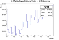
| + | Below is the histogram representing the time cuts for the 4th run | ||
| + | |||
| + | [[File:0 04Percent SeSage TimeCuts 1DHistogram Run4.png|200px]] | ||
| + | |||
| + | Below are the time cuts | ||
| + | |||
| + | 0-300 (Pure Se) | ||
| + | |||
| + | 306-359 (Co-60) | ||
| + | |||
| + | 362-818 (Mixture) | ||
=Gamma Spectrum Analysis= | =Gamma Spectrum Analysis= | ||
| + | ==50% Sample Analysis== | ||
| + | Below is the analysis table for the 50% Se/Sage mixture. The 103 keV line of Se-81m corresponds to a channel # of 130. Due to the sloppiness of the spectrum, I will use a linear + Gaussian fitting function and restrict my analysis to 6 channels because there are other energy lines nearby. Below is a sample spectrum for an idea of the resolution of Detector B for this measurement | ||
| + | |||
| + | [[File:LB 50Percent SeSage SampleSpectrum.png|200px]] | ||
| + | |||
| + | As a comparison for the constant fit, here is a sample spectrum of the Se/Sage measured by Detector A | ||
| + | |||
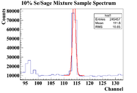
| + | [[File:10Percent SeSage SampleSpectrum.png|200px]] | ||
| + | |||
| + | |||
| + | {| border="3" cellpadding="5" cellspacing="0" | ||
| + | || || 0<t<300 || | ||
| + | |- | ||
| + | ||Thin Window Histogram || | ||
| + | |- | ||
| + | ||Signal in Thin Window || | ||
| + | |- | ||
| + | ||Integrated Background || | ||
| + | |- | ||
| + | ||Signal - Background || | ||
| + | |- | ||
| + | ||Runtime (s) || | ||
| + | |- | ||
| + | ||Rate (Hz) || | ||
| + | |- | ||
| + | ||Integral Decay Correction (Hz) || | ||
| + | |- | ||
| + | ||Dead Time (%) || | ||
| + | |- | ||
| + | ||Dead Time Corrected Signal (Hz) || | ||
| + | |- | ||
| + | ||.Dat File Entry For HL Plot || | ||
| + | |} | ||
==10% Sample Analysis== | ==10% Sample Analysis== | ||
Below is the analysis table for the 10% Se/Sage mixture. The 103 keV line of Se-81m corresponds to a channel # of 113 | Below is the analysis table for the 10% Se/Sage mixture. The 103 keV line of Se-81m corresponds to a channel # of 113 | ||
| + | |||
{| border="3" cellpadding="5" cellspacing="0" | {| border="3" cellpadding="5" cellspacing="0" | ||
| − | ||0<t<300 || 730<t<1020 || 1480<t<1775 || 2250<t<2550 || 3050<t<3300 || 3775<t<4050 || 4480<t<4770 | + | || || 0<t<300 || 730<t<1020 || 1480<t<1775 || 2250<t<2550 || 3050<t<3300 || 3775<t<4050 || 4480<t<4770 |
|- | |- | ||
| − | ||Thin Window Histogram || | + | ||Thin Window Histogram || [[File:10Percent SeSageMix 0 t 300Sec 10Chan Se81m.png|200px]] || [[File:10Percent SeSageMix 730 t 1020Sec 10Chan Se81m.png|200px]] || [[File:10Percent SeSageMix 1480 t 1775Sec 10Chan Se81m.png|200px]] || [[File:10Percent SeSageMix 2250 t 2550Sec 10Chan Se81m.png|200px]] || [[File:10Percent SeSageMix 3050 t 3300Sec 10Chan Se81m.png|200px]] || [[File:10Percent SeSageMix 3775 t 4050Sec 10Chan Se81m.png|200px]] || [[File:10Percent SeSageMix 4480 t 4770Sec 10Chan Se81m.png|200px]] |
|- | |- | ||
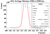
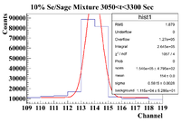
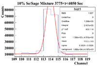
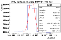
| − | ||Signal in Thin Window || | + | ||Signal in Thin Window || <math> 6.019 \times 10^5 \pm 775.82</math> || <math> 4.852 \times 10^5 \pm 696.56 </math> || <math> 4.161 \times 10^5 \pm 645.06 </math> || <math> 3.667 \times 10^5 \pm 605.56 </math> || <math> 2.645 \times 10^5 \pm 514.30 </math> || <math> 2.451 \times 10^5 \pm 495.08 </math> || <math> 2.344 \times 10^5 \pm 484.15 </math> |
|- | |- | ||
| − | ||Integrated Background || | + | ||Integrated Background || <math> 2.956 \times 10^5 \pm 885.1 </math> || <math> 2.074 \times 10^5 \pm 728.7 </math> || <math> 1.668 \times 10^5 \pm 653.0 </math> || <math> 1.47 \times 10^5 \pm 606.0 </math> || <math> 1.115 \times 10^5 \pm 528.6 </math> || <math> 1.055 \times 10^5 \pm 418.7 </math> || <math> 9.935 \times 10^4 \pm 496 </math> |
|- | |- | ||
| − | ||Signal - Background || | + | ||Signal - Background || <math> 3.063 \times 10^5 \pm 1177.01 </math> || <math> 2.778 \times 10^5 \pm 1008.07 </math> || <math> 2.493 \times 10^5 \pm 917.88</math> || <math> 2.197 \times 10^5 \pm 856.70 </math> || <math> 1.53 \times 10^5 \pm 737.51 </math> || <math> 1.396 \times 10^5 \pm 648.39 </math> || <math> 1.35050 \times 10^5 \pm 693.12 </math> |
|- | |- | ||
| − | ||Runtime (s) || 300 || 290 || 295 || 300 || 250 || 275 | + | ||Runtime (s) || 300 || 290 || 295 || 300 || 250 || 275 || 290 |
|- | |- | ||
| − | ||Rate (Hz) || | + | ||Rate (Hz) || <math> 1021 \pm 3.92 </math> || <math> 957.93 \pm 3.48 </math> || <math> 845.08 \pm 3.11 </math> || <math> 732.33 \pm 2.86 </math> || <math> 612 \pm 2.95 </math> || <math> 507.64 \pm 2.36 </math> || <math> 465.69 \pm 2.39 </math> |
|- | |- | ||
| − | ||Integral Decay Correction (Hz) || | + | ||Integral Decay Correction (Hz) || <math> 1052.2 \pm 4.04 </math> || <math> 986.23 \pm 3.58 </math> || <math> 870.47 \pm 3.20 </math> || <math> 754.71 \pm 2.95 </math> || <math> 627.56 \pm 3.03 </math> || <math> 521.85 \pm 2.43 </math> || <math> 479.44 \pm 2.46 </math> |
|- | |- | ||
| − | ||Dead Time (%) || | + | ||Dead Time (%) || 5.06 +/- 0.39 || 3.06 +/- 0.30 || 2.53 +/- 0.31 || 2.26 +/- 0.33 || 1.92 +/- 0.26 || 1.65 +/- 0.34 || 1.55 +/- 0.18 |
|- | |- | ||
||Dead Time Corrected Signal (Hz) || | ||Dead Time Corrected Signal (Hz) || | ||
| Line 302: | Line 414: | ||
||.Dat File Entry For HL Plot || | ||.Dat File Entry For HL Plot || | ||
|} | |} | ||
| + | |||
| + | ===Background and SNR Information=== | ||
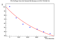
| + | Below is a plot of the background in a 10 channel window around the short lived half life's energy peak of interest (103 keV). The long lived half live can be measured for at least a year even in a 0.1% by mass concentration, so it is less pressing. The values presented are weighted by the mass of the sage ash. | ||
| + | |||
| + | [[File:LB 10Percent OvenAshSeMix BackgroundExpoHL.png|200px]] | ||
| + | |||
| + | The fit parameters are | ||
| + | |||
| + | Constant: 4.50734e+00 +/- 2.42037e-03 | ||
| + | |||
| + | Slope: -2.31438e-04 +/- 1.05610e-06 | ||
| + | |||
| + | Which gives a rough half life of 49.92 +/- 0.23 minutes | ||
| + | |||
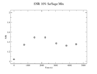
| + | Below is the SNR plotted in xmgrace | ||
| + | |||
| + | [[File:LB SNR 10Percent SeSageMix.png|200px]] | ||
==0.1% Sample Analysis== | ==0.1% Sample Analysis== | ||
| Line 335: | Line 464: | ||
{| border="3" cellpadding="5" cellspacing="0" | {| border="3" cellpadding="5" cellspacing="0" | ||
| − | || || 0<t<290 || | + | || || 0<t<290 || 0<t<300 (Run 2) || 740<t<1020 (Run 2) |
|- | |- | ||
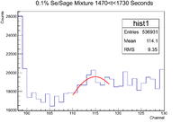
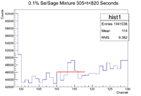
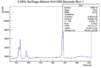
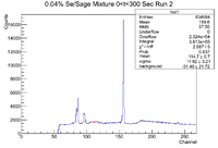
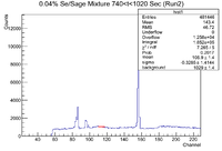
| − | ||Thin Window Histogram || [[File:0 04Percent SeSage Mix 0 t 290Sec Run1.png|200px]] | + | ||Thin Window Histogram || [[File:0 04Percent SeSage Mix 0 t 290Sec Run1.png|200px]] || [[File:0 04Percent SeSage Mix 0 t 300Sec Run2.png|200px]] || [[File:0 04Percent SeSage Mix 740 t 1020Sec Run2.png|200px]] |
|- | |- | ||
| − | ||Signal in Thin Window || No Signal Visible | + | ||Signal in Thin Window || No Signal Visible || No Signal Visible || No Signal Visible |
|- | |- | ||
||Integrated Background || - || - || - || - | ||Integrated Background || - || - || - || - | ||
| Line 345: | Line 474: | ||
||Signal - Background || - || - || - || - | ||Signal - Background || - || - || - || - | ||
|- | |- | ||
| − | ||Runtime (s) || 290 | + | ||Runtime (s) || 290 || 300 || 280 |
|- | |- | ||
||Rate (Hz) || - || - || - || - | ||Rate (Hz) || - || - || - || - | ||
| Line 357: | Line 486: | ||
||.Dat File Entry For HL Plot || - || - || - || - | ||.Dat File Entry For HL Plot || - || - || - || - | ||
|} | |} | ||
| + | |||
| + | ===Background and SNR Information=== | ||
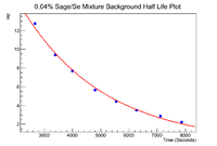
| + | Below is the information for the background in the window [109,119] (Channel # here). The data was weighted by both the runtime and the mass of the sage ash. | ||
| + | |||
| + | [[File:0 04Percent SageSeMixture BackgroundHL.png|200px]] | ||
| + | |||
| + | The fit parameters here are | ||
| + | |||
| + | Constant: 3.42624e+00 +/- 3.71043e-03 | ||
| + | |||
| + | Slope: -3.44115e-04 +/- 7.67333e-07 | ||
| + | |||
| + | which gives a half life of 33.57 +/- 0.07 minutes. | ||
| + | |||
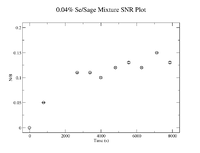
| + | The SNR plot is shown below | ||
| + | |||
| + | [[File:LB 0 04Percent SNRPlot xmgrace.png|200px]] | ||
| + | |||
| + | =Fall 2018 Possible Sage Irradiation Activity Prediction= | ||
| + | |||
| + | Isotope Search link: http://nucleardata.nuclear.lu.se/toi/ | ||
| + | |||
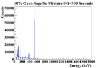
| + | For this section I will attempt to identify the most active line within a sagebrush sample. The histograms that follow in this section will be weighted by the mass of the sage that was used for the sample. I will use the 10% Sage/Se mixture because it was processed using the oven method for dehydration. The mass was 0.5111g which gives a weighting factor of 1.9566 <math> g^{-1} </math> Below is a full spectrum for the time cut of 0 <t< 300 seconds. | ||
| + | |||
| + | [[File:10Percent SeSageMix 0 t 300Sec FullSpectrum PreIrrAnalysis.png|200px]] | ||
| + | |||
| + | [[File:10Percent SeSageMix 0 t 300Sec 0 E 600 PreIrrAnalysis.png|200px]] | ||
| + | [[File:10Percent SeSageMix 0 t 300Sec 600 E 1500 PreIrrAnalysis.png|200px]] | ||
| + | |||
| + | It seems the two most prominent lines are around 150 keV and 250 keV, so let's try to study the decay of those first. | ||
| + | |||
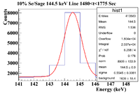
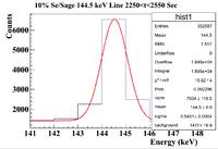
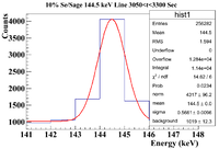
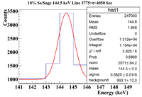
| + | ==144.5 keV Line== | ||
| + | |||
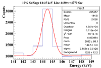
| + | Note: the x-axis for the first 2 histograms should be Energy (keV). This line is NOT present in the Pure Se Sample, so it should be a line produced by the sage itself. | ||
| + | |||
| + | {| border="3" cellpadding="5" cellspacing="0" | ||
| + | || || 0<t<300 || 730<t<1020 || 1480<t<1775 || 2250<t<2550 || 3050<t<3300 || 3775<t<4050 || 4480<t<4770 | ||
| + | |- | ||
| + | || Histogram || [[File:10Percent SeSageMix 0 t 300Sec 144keVLine PreIrrAnalysis.png|200px]] || [[File:10Percent SeSageMix 730 t 1020Sec 144keVLine PreIrrAnalysis.png|200px]] || [[File:10Percent SeSageMix 1480 t 1775Sec 144keVLine PreIrrAnalysis.png|200px]] || [[File:10Percent SeSageMix 2250 t 2550Sec 144keVLine PreIrrAnalysis.png|200px]] || [[File:10Percent SeSageMix 3050 t 3300Sec 144keVLine PreIrrAnalysis.png|200px]] || [[File:10Percent SeSageMix 3775 t 4050Sec 144keVLine PreIrrAnalysis.png|200px]] || [[File:10Percent SeSageMix 4480 t 4770Sec 144keVLine PreIrrAnalysis.png|200px]] | ||
| + | |- | ||
| + | ||Signal in Thin Window || 3.424 <math> \times 10^4 \pm </math> 185.04 || 2.535 <math> \times 10^4 \pm </math> 159.22 || 2.037 <math> \times 10^4 \pm </math> 142.72 || 1.695 <math> \times 10^4 \pm </math> 130.19 || 1.14 <math> \times 10^4 \pm </math> 106.77 || 1.154 <math> \times 10^4 \pm </math> 107.42 || 1.115 <math> \times 10^4 \pm </math> 105.59 | ||
| + | |- | ||
| + | ||Integrated Background || 1.9628 <math> \times 10^4 \pm </math> 167.4 || 1.4035 <math> \times 10^4 \pm </math> 139.3 || 1.1473 <math> \times 10^4 \pm </math> 128.80 || 9877 <math> \pm </math> 118.3 || 7133 <math> \pm </math> 86.1 || 6951.7 <math> \pm </math> 84.0 || 7182 <math> \pm </math> 85.4 | ||
| + | |- | ||
| + | ||Signal - Background || 1.4612 <math> \times 10^4 \pm </math> 249.52 || 1.1315 <math> \times 10^4 \pm </math> 211.55 || 8897 <math> \pm </math> 192.24 || 7073 <math> \pm </math> 175.91 || 4267 <math> \pm </math> 137.16 || 4588.3 <math> \pm </math> 136.36 || 3968 <math> \pm </math> 135.80 | ||
| + | |- | ||
| + | ||Runtime (s) || 300 || 290 || 295 || 300 || 250 ||275 || 290 | ||
| + | |- | ||
| + | ||Rate (Hz) || 48.71 <math>\pm</math> 0.83 || 39.02 <math> \pm </math> 0.73 || 30.16 <math> \pm </math> 0.65 || 23.58 <math> \pm </math> 0.59 || 17.07 <math> \pm </math> 0.55 || 16.68 <math> \pm </math> 0.49 || 13.68 <math> \pm </math> 0.47 | ||
| + | |} | ||
| + | |||
| + | Without any corrections, the half life here is 38.61 <math> \pm </math> 0.84 minutes. This is likely Cl-34m (32 min half life) produced by a (g,n) reaction on Cl-35 (75.76% natural abundance), which is stable, because a second line characteristic of Cl-34m was found (1176 keV). This could also be produced by a (g,pn) knockout on Ar-36 in air. This is chlorine since using the isotope search with an energy uncertainty of 5 keV and a half life uncertainty of 10 minutes, the only isotope that shared 146 and 1176 keV with branching ratios that made sense was Cl-34m. | ||
| + | |||
| + | |||
| + | =9/10/18 Irradiation= | ||
| + | The mass information is | ||
| + | |||
| + | Al Cylinder: 26.0249g | ||
| + | |||
| + | Sage Ash (oven method): 2.0913g | ||
| + | |||
| + | Beam off: 18:30 | ||
| + | |||
| + | ==Calibration== | ||
| + | Below is the runlist used for the calibration on Detector D | ||
| + | |||
| + | |||
| + | {| border="3" cellpadding="5" cellspacing="0" | ||
| + | || Source || Serial No. || Reference Date || Activiy || Half life || Expected Energies (keV) || Line Seen (Channel No.) || Runtime (s) || Position || File Name || Date Measured | ||
| + | |- | ||
| + | || Mn-54 || J4-348 || 8/1/12 || 9.882 uCi || 312.20 days || 834.827 || 835.117 || 300.601 || 10 || LB_Mn_54_9_10_18_Pos10_DetD || 9/10/18 | ||
| + | |- | ||
| + | ||Cs-137 || 129793 || 7/1/08 || 1.066 uCi || 30.08 years || 661.657 || 661.887 || 141.356 || 10 || LB_Cs137_9_10_18_Pos010_DetD || 9/10/18 | ||
| + | |- | ||
| + | ||Co-60 || 129739 || 07/01/08 || 1.082 uCi || 1925.28 days || 1173.228, 1332.492 || 1173.338, 1332.564 ||232.521 || 10 || LB_Co60_9_10_18_Pos010_DetD || 9/10/18 | ||
| + | |- | ||
| + | ||Ba-133 || 129790 || 07/01/08 || 1.188 uCi || 10.551 years ||80.9979, 276.3989, 302.8508, 356.0129, 383.8485 || 81.391, 276.741, 303.166, 356.315, 384.137 ||250.816 ||10 || LB_Ba133_9_10_18_Pos010_DetD || 9/10/18 | ||
| + | |- | ||
| + | |} | ||
| + | |||
| + | The calibration coefficients are (according to my fits) | ||
| + | |||
| + | Intercept = -0.370972 +/- 0.616 | ||
| + | |||
| + | Slope = 0.490352 +/- 0.000534241 | ||
| + | |||
| + | The calibration used at the IAC was | ||
| + | |||
| + | Intercept = 0.272366 | ||
| + | |||
| + | Slope = 0.490198 | ||
| + | |||
| + | ==Efficiency== | ||
| + | Below is a table of the runlist used for the efficiency on Detector D. | ||
| + | |||
| + | {| border="3" cellpadding="5" cellspacing="0" | ||
| + | || Source || Serial No. || Reference Date || Activiy || Half life || Expected Energies (keV) ||Start || Stop|| Runtime (s) || Position ||File Name || Date Measured | ||
| + | |- | ||
| + | || Mn-54 || J4-348 || 8/1/12 || 9.882 uCi || 312.20 days || 828.859 ||12:45 || 12:50|| 300.601 || 10 || LB_Mn_54_9_10_18_Pos10_DetD || 9/10/18 | ||
| + | |- | ||
| + | ||Mn-54 || J4-348 || 8/1/12 || 9.882 uCi || 312.20 days || 828.859 || 12:52 || 12:57 || 305.787 || 20 || LB_Mn_54_9_10_Pos020_DetD || 9/10/18 | ||
| + | |- | ||
| + | ||Mn-54 || J4-348 || 8/1/12 || 9.882 uCi || 312.20 days || 828.859 ||12:59:41 ||113:04 ||300.734 || 30 || LB_Mn_54_9_10_18_Pos030_DetD || 9/10/18 | ||
| + | |- | ||
| + | ||Co-60 || 129740 || 07/01/08 || 10.42 uCi || 1925.28 days || 1173.228, 1332.492 || 18:17:35 ||18:24 || 409.011 || 80 || LB_Co60_9_10_18_Pos080_DetD || 9/10/18 | ||
| + | |- | ||
| + | ||Co-60 || 129740 || 07/01/08 || 10.42 uCi || 1925.28 days || 1173.228, 1332.492 || 18:26:11 || 18:29 || 201.084 || 70 || LB_Co60_9_10_18_Pos070_DetD || 9/10/18 | ||
| + | |- | ||
| + | |} | ||
| + | |||
| + | ==Runlist for 9/10/18 Irradiated Samples== | ||
| + | |||
| + | {| border="3" cellpadding="5" cellspacing="0" | ||
| + | || Sample || Date || Start || Stop || Runtime (s) || Position || Detector || % Dead || File Name | ||
| + | |- | ||
| + | || Sage Ash || 9/10/18 ||20:31:35 || 09:26 || 46507.875 || 40 || Detector D || < 2% || LB_SageAsh_OvenMethod_9_10_18_DetD_002 | ||
| + | |- | ||
| + | ||Sage Ash || 9/11/18 || 14:59:50 || 10:57 || 71854.534 || 40 || Detector D || <1% || LB_SageAsh_OvenMethod_9_11_18_DetD_003 | ||
| + | |- | ||
| + | || Sage Ash || 9/12/18 || 11:01:05 || ||89908.033 || 20 || Detector D || <1% || LB_SageAsh_OvenMethod_9_12_18_DetD_Pos20_001 | ||
| + | |- | ||
| + | || Sage Ash || 9/13/18 || 12:03:02 || || 73275.295 || 10 || Det D || <1% || LB_SageAsh_OvenMethod_9_13_18_DetD_Pos10_001 | ||
| + | |- | ||
| + | || Sage Ash || 9/14/18 || 09:26:37 || 10:41 (9/17/18) || || 10 || Det D || <1% || LB_SageAsh_OvenMethod_9_14_18_DetD_Pos10_001 | ||
| + | |- | ||
| + | || Sage Ash || 9/17/18 || 10:51:02 || || || 10 || Det D || <1% || LB_SageAsh_OvenMethod_9_17_18_DetD_Pos10_001 | ||
| + | |- | ||
| + | || Sage Ash || 10/01/18 ||14:04:00 || || || Face of Detector || Det D || <1% || LB_SageAsh_OvenMethod_10_1_18_DetD_DetFace_002 | ||
| + | |- | ||
| + | |} | ||
| + | |||
| + | =September Sage+Al Analysis= | ||
| + | |||
| + | https://wiki.iac.isu.edu/index.php/MCNP_Sim_of_Jack_Converter | ||
| + | |||
| + | Below is the first measured histogram generated from the file LB_SageAsh_OvenMethod_9_10_18_DetD_002. Note that the Al cylinder and the sage ash were not separated, so there will be some lines from Al present. The histogram shown below is not weighted because there are two different samples in front of the detector at the same time (Al cylinder and sage ash). Once the lines have been identified, the mass will be taken into account | ||
| + | |||
| + | The command lines used in the directory /data/IAC/LB_Thesis_Analysis/Sept2018_SageAshBackground/Samples | ||
| + | |||
| + | .L Eff.C | ||
| + | |||
| + | Eff t | ||
| + | |||
| + | t.Loop(RangeMin,RangeMax); | ||
| + | |||
| + | |||
| + | [[File:LB SageAshOven 9 10 18 FirstMeasure.png|200px]] | ||
| + | |||
| + | |||
| + | Below is a histogram of the second measurement taken overnight on 9/11/18 | ||
| + | |||
| + | [[File:LB SageAshOven 9 11 18 SecondMeasure.png|200px]] | ||
| + | |||
| + | Now let's overlay these two histograms as a function of activity rather than counts to see if there are any lines that have decayed away that could possibly be identified. I did this as Hz vs. 0.5*(Chan)-0.4. The dithering proved to be quite difficult for both histograms. | ||
| + | |||
| + | [[File:LB SageAshOven Measure1and2 Overlay.png|200px]] | ||
| + | |||
| + | Below is a table detailing the decaying/decayed lines. The relative rates were calculated using a linear fit plus a Gaussian fit, then the background subtracted activity was found. | ||
| + | |||
| + | |||
| + | {| border="3" cellpadding="5" cellspacing="0" | ||
| + | || Line Seen (keV) || Isotope | ||
| + | |- | ||
| + | ||846 || Mn-56 | ||
| + | |- | ||
| + | || 1810 || Mn-56 | ||
| + | |- | ||
| + | || 2133 || Mn-56 | ||
| + | |- | ||
| + | ||1368 || Na-24 | ||
| + | |- | ||
| + | ||2754 || Na-24 | ||
| + | |- | ||
| + | |} | ||
| + | |||
| + | ==Background Analysis== | ||
| + | Below is the analysis of the background around the Se line of interest. The histograms were unweighted due to the presence of both the Al cylinder and the sage ash. The data points on the half life plot are weighted by the runtime. The energy window used was [90,130]. The times I concerned myself with spanned 5 half lives of Se (17184 sec) which were split cut into 10 different sets (runtime = 1718.4 sec). | ||
| + | |||
| + | The parameters are as follows | ||
| + | |||
| + | |||
| + | {| border="3" cellpadding="5" cellspacing="0" | ||
| + | || || 0<t<1718.4 s || 1718.4<t<3436.8 s || 3436.8<t<5155.2 s || 5155.2<t<6873.6 s || 6873.6<t<8592 s || 8592<t<10310.4 s || 10310.4<t<12028.8 s || 12028.8<t<13747.2 s || 13747.2<t<15461.6 s || 15461.6<t<17180 s | ||
| + | |- | ||
| + | || Slope (<math> \alpha </math>) || 5.853 <math> \pm </math> 0.562 || 5.33 <math> \pm </math> 0.54 || 4.981 <math> \pm </math> 0.532 || 5.423 <math> \pm </math> 0.521 || 6.234 <math> \pm </math> 0.511 || 5.155 <math> \pm </math> 0.503 || 4.703 <math> \pm </math> 0.496 || 4.053 <math> \pm </math> 0.489 || 4.49 <math> \pm </math> 0.49 || 4.506 <math> \pm </math> 0.503 | ||
| + | |- | ||
| + | || Intercept (<math> \beta </math> ) || 1051 <math> \pm </math> 61.9 || 998.8 <math> \pm </math> 59.6 || 974.6 <math> \pm </math> 58.7 || 871.7 <math> \pm </math> 57.4 || 731.4 <math> \pm </math> 56.2 || 796.7 <math> \pm </math> 55.4 || 807.3 <math> \pm </math> 54.6 || 841 <math> \pm </math> 53.9 || 836.8 <math> \pm </math> 54.5 || 868.6 <math> \pm </math> 55.4 | ||
| + | |- | ||
| + | ||Integral from [90,130] || 39.45 <math> \pm </math> 2.04 || 36.90 <math> \pm </math> 1.96 || 35.44 <math> \pm </math> 1.92 || 34.18 <math> \pm </math> 1.89 || 32.99 <math> \pm </math> 1.85 || 31.74 <math> \pm </math> 1.82 || 30.83 <math> \pm </math> 1.80 || 29.95 <math> \pm </math> 1.77 || 30.98 <math> \pm </math> 1.78 || 31.76 <math> \pm </math> 1.82 | ||
| + | |- | ||
| + | |} | ||
| + | |||
| + | |||
| + | |||
| + | Now the total background was found by integrating the linear fit function across the region of interest, in other words | ||
| + | |||
| + | <math> f(x) = \int_a^b (\alpha x + \beta)dx </math> | ||
| + | |||
| + | To find the error in the integral, use the standard error propagation method | ||
| + | |||
| + | <math> \sigma_f = \sqrt{(\frac{\partial f}{\partial \alpha})^2 \sigma_{\alpha}^2 + (\frac{\partial f}{\partial \beta})^2 \sigma_{\beta}^2} </math> | ||
| + | |||
| + | <math> = \sqrt{[\frac{\partial}{\partial \alpha}(\int_a^b (\alpha x + \beta)dx)]^2 \sigma_{\alpha}^2 + [\frac{\partial}{\partial \beta}(\int_a^b (\alpha x + \beta)dx)]^2 \sigma_{\beta}^2} </math> | ||
| + | |||
| + | Since the partial derivatives are not taken with respect to the variable of integration and the function is analytic within the region, the derivative may be moved inside the integral. This action yields | ||
| + | |||
| + | <math>\sigma_f = \sqrt{(\int_a^b x dx)^2 \sigma_{\alpha}^2 + (\int_a^b dx)^2 \sigma_{\beta}^2} </math> | ||
| + | |||
| + | <math> = \sqrt{(\frac{b^2-a^2}{2})^2 \sigma_{\alpha}^2 + (b-a)^2 \sigma_{\beta}^2} </math> | ||
| + | |||
| + | |||
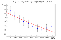
| + | Below is the initial plot of the background in the region from [90,130] | ||
| + | |||
| + | [[File:LB Sept2018 Sage Al BackgroundHL InitialPlot.png|200px]] | ||
| + | |||
| + | This plot has some outliers and fluctuations in the background that could be due to the presence of other sources (Dr. Dale was measuring very hot gallium on Det A during my overnight measurement). | ||
| + | |||
| + | ===10 Channel Analysis=== | ||
| + | The fits were done in a larger window [90,130] to get enough bins for a good fit, so I should be able to simply change the bounds of the integration to make the correction. There is definitely some randomness within the time cuts which produce bins with data above and below the fit line, which makes this more difficult. With the dithering, the peak on Detector A has a mean value of 103.949 kev, so the window I will analyze on Detector D (calibrated to energy) will be [99,109] keV | ||
| + | |||
| + | |||
| + | {| border="3" cellpadding="5" cellspacing="0" | ||
| + | || || 0<t<1718.4 s || 1718.4<t<3436.8 s || 3436.8<t<5155.2 s || 5155.2<t<6873.6 s || 6873.6<t<8592 s || 8592<t<10310.4 s || 10310.4<t<12028.8 s || 12028.8<t<13747.2 s || 13747.2<t<15461.6 s || 15461.6<t<17184 s || 17184 <t< 18902.4 s || 18902.4 <t< 20620.8 s || 20620.8<t<22339.2 s || 22339.2<t<24057.6 s || 24057.6<t<25776 s || 25776<t<27494.4 s || 27494.4<t<29212.8 s || 29212.8 <t< 30931.2 s || 30931.2 <t< 32649.6 s || 32649.6<t<34368 s || 34368<t<36086.4 s || 36086.4<t<37804.8 || 37804.8 <t< 39523.2 || 39523.2<t<41241.6 s || 41241.6 <t< 42960 s || 42960<t<44678.4 s || 44678.4 <t< 46396.8 s | ||
| + | |- | ||
| + | || Slope (<math> \alpha </math>) || 5.853 <math> \pm </math> 0.562 || 5.33 <math> \pm </math> 0.54 || 4.981 <math> \pm </math> 0.532 || 5.423 <math> \pm </math> 0.521 || 6.234 <math> \pm </math> 0.511 || 5.155 <math> \pm </math> 0.503 || 4.703 <math> \pm </math> 0.496 || 4.053 <math> \pm </math> 0.489 || 4.49 <math> \pm </math> 0.49 || 4.506 <math> \pm </math> 0.503 || 5.101 <math> \pm </math> 0.496 || 5.215 <math> \pm </math> 0.490 || 4.695 <math> \pm </math> 0.482 || 4.685 <math> \pm </math> 0.477 || 4.731 <math> \pm </math> 0.468 || 4.218 <math> \pm </math> 0.468 || 3.95 <math> \pm </math> 0.459 || 4.388 <math> \pm </math> 0.452 || 4.180 <math> \pm </math> 0.446 || 3.512 <math> \pm </math> 0.442 || 4.423 <math> \pm </math> 0.440 || 4.751 <math> \pm </math> 0.435 || 3.695 <math> \pm </math> 0.431 || 3.372 <math> \pm </math> 0.424 || 3.112 <math> \pm </math> 0.420 || 3.784 <math> \pm </math> 0.415 || 2.792 <math> \pm </math> 0.414 | ||
| + | |- | ||
| + | || Intercept (<math> \beta </math> ) || 1051 <math> \pm </math> 61.9 || 998.8 <math> \pm </math> 59.6 || 974.6 <math> \pm </math> 58.7 || 871.7 <math> \pm </math> 57.4 || 731.4 <math> \pm </math> 56.2 || 796.7 <math> \pm </math> 55.4 || 807.3 <math> \pm </math> 54.6 || 841 <math> \pm </math> 53.9 || 836.8 <math> \pm </math> 54.5 || 868.6 <math> \pm </math> 55.4 || 769.5 <math> \pm </math> 54.6 || 732.8 <math> \pm </math> 54.0 || 737.5 <math> \pm </math> 53.1 || 715.1 <math> \pm </math> 52.6 || 673.8 <math> \pm </math> 51.6 || 714.3 <math> \pm </math> 51.5 || 701.0 <math> \pm </math> 50.6 || 625.5 <math> \pm </math> 49.8 || 620.9 <math> \pm </math> 49.1 || 676.1 <math> \pm </math> 48.8 || 562.8 <math> \pm </math> 48.4 || 508.3 <math> \pm </math> 47.9 || 600.2 <math> \pm </math> 47.5 || 608 <math> \pm </math> 46.7 || 623 <math> \pm </math> 46.3 || 519.5 <math> \pm </math> 45.7 || 618.1 <math> \pm </math> 45.6 | ||
| + | |- | ||
| + | ||Fit Function Integral from [99,109] || 9.67 <math> \pm </math> 0.50 || 9.04 <math> \pm </math> 0.48 || 8.69 <math> \pm </math> 0.47 || 8.35 <math> \pm </math> 0.46 || 8.03 <math> \pm </math> 0.45 || 7.76 <math> \pm </math> 0.44 || 7.54 <math> \pm </math> 0.44 || 7.35 <math> \pm </math> 0.43 || 7.59 <math> \pm </math> 0.43 || 7.78 <math> \pm </math> 0.44 || 7.57 <math> \pm </math> 0.44 || 7.42 <math> \pm </math> 0.43 || 7.13 <math> \pm </math> 0.42 || 7.00 <math> \pm </math> 0.42 || 6.78 <math> \pm </math> 0.41 || 6.71 <math> \pm </math> 0.41 || 6.47 <math> \pm </math> 0.40 || 6.30 <math> \pm </math> 0.40 || 6.14 <math> \pm </math> 0.39 || 6.06 <math> \pm </math> 0.39 || 5.95 <math> \pm </math> 0.39 || 5.83 <math> \pm </math> 0.38 || 5.73 <math> \pm </math> 0.38 || 5.58 <math> \pm </math> 0.37 || 5.51 <math> \pm </math> 0.37 || 5.31 <math> \pm </math> 0.37 || 5.29 <math> \pm </math> 0.36 | ||
| + | |- | ||
| + | ||Stats Box Integral || <math> 1.674 \times 10^4 </math> || <math> 1.565 \times 10^4 </math> || <math> 1.505 \times 10^4 </math> || <math> 1.159 \times 10^4 </math> || <math> 1.401 \times 10^4 </math> || <math> 1.341 \times 10^4 </math> || <math> 1.306 \times 10^4 </math> || <math> 1.292 \times 10^4 </math> || <math> 1.332 \times 10^4 </math> || <math> 1.347 \times 10^4 </math> || <math> 1.313 \times 10^4 </math> || <math> 1.296 \times 10^4 </math> || <math> 1.238 \times 10^4 </math> || <math> 1.197 \times 10^4 </math> || <math> 1.194 \times 10^4 </math> || <math> 1.166 \times 10^4 </math> || <math> 1.134 \times 10^4 </math> || <math> 1.101 \times 10^4 </math> || <math> 1.085 \times 10^4 </math> || <math> 1.064 \times 10^4 </math> || <math> 1.046 \times 10^4 </math> || <math> 1.027 \times 10^4 </math> || 9943 || 9872 || 9699 || 9206 || 9110 | ||
| + | |- | ||
| + | ||Stats Box Activity (Hz) || 9.58 <math> \pm </math> 0.07 || 9.12 <math> \pm </math> 0.07 || 8.76 <math> \pm </math> 0.07 || 6.74 <math> \pm </math> 0.06 || 8.15 <math> \pm </math> 0.07 || 7.80 <math> \pm </math> 0.07 || 7.60 <math> \pm </math> 0.07 || 7.53 <math> \pm </math> 0.07 || 7.75 <math> \pm </math> 0.07 || 7.84 <math> \pm </math> 0.07 || 7.64 <math> \pm </math> 0.07 || 7.54 <math> \pm </math> 0.07 || 7.20 <math> \pm </math> 0.06 || 6.97 <math> \pm </math> 0.06 || 6.95 <math> \pm </math> 0.06 || 6.79 <math> \pm </math> 0.06 || 6.60 <math> \pm </math> 0.06 || 6.41 <math> \pm </math> 0.06 || 6.31 <math> \pm </math> 0.06 || 6.19 <math> \pm </math> 0.06 || 6.09 <math> \pm </math> 0.06 || 5.98 <math> \pm </math> 0.06 || 5.79 <math> \pm </math> 0.06 || 5.74 <math> \pm </math> 0.06 || 5.64 <math> \pm </math> 0.06 || 5.36 <math> \pm </math> 0.06 || 5.30 <math> \pm </math> 0.06 | ||
| + | |- | ||
| + | ||Corrected Background Measurement || 9.58 <math> \pm </math> 0.09 || 9.12 <math> \pm </math> 0.08 || 8.76 <math> \pm </math> 0.07 || 6.74 <math> \pm </math> 1.61 || 8.15 <math> \pm </math> 0.12 || 7.80 <math> \pm </math> 0.04 || 7.60 <math> \pm </math> 0.06 || 7.53 <math> \pm </math> 0.18 || 7.75 <math> \pm </math> 0.16 || 7.84 <math> \pm </math> 0.06 || 7.64 <math> \pm </math> 0.07 || 7.54 <math> \pm </math> 0.12 || 7.20 <math> \pm </math> 0.07 || 6.97 <math> \pm </math> 0.03 || 6.95 <math> \pm </math> 0.17 || 6.79 <math> \pm </math> 0.08 || 6.60 <math> \pm </math> 0.13 || 6.41 <math> \pm </math> || 6.31 <math> \pm </math> 0.17 || 6.19 <math> \pm </math> 0.13 || 6.09 <math> \pm </math> 0.14 || 5.98 <math> \pm </math> 0.15 || 5.79 <math> \pm </math> 0.06 || 5.74 <math> \pm </math> 0.16 || 5.64 <math> \pm </math> 0.13 || 5.36 <math> \pm </math> 0.05 || 5.30 <math> \pm </math> 0.01 | ||
| + | |- | ||
| + | |} | ||
| + | |||
| + | |||
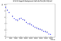
| + | [[File:LB Sept2018 Sage Al BackgroundHL InitialPlot 10Chan_Full.png|200px]] | ||
| + | |||
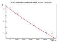
| + | This looks like there are two separate half lives present, so split them up and fit. | ||
| + | |||
| + | [[File:LB Sept2018 Sage Al BackgroundHL InitialPlot 10Chan FirstPortion.png|200px]] | ||
| + | |||
| + | The fit parameters for the first portion are | ||
| + | |||
| + | Slope: -2.22732e-05 +/- 8.61118e-07 | ||
| + | |||
| + | Constant:2.25058e+00 +/- 6.19036e-03 | ||
| + | |||
| + | Which gives a half life of 8.47 +/- 0.32 hours | ||
| + | |||
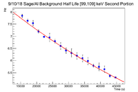
| + | [[File:LB Sept2018 Sage Al BackgroundHL InitialPlot 10Chan SecondPortion.png|200px]] | ||
| + | |||
| + | The fit parameters for the second portion are | ||
| + | |||
| + | Constant: 2.24079e+00 +/- 5.78712e-03 | ||
| + | |||
| + | Slope: -1.28411e-05 +/- 1.46816e-07 | ||
| + | |||
| + | Which gives a half life of 14.99 +/- 0.17 hours | ||
| + | |||
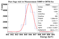
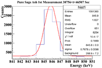
| + | ==846 keV Line Analysis== | ||
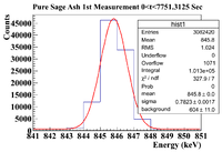
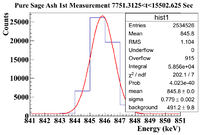
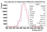
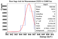
| + | Below is the analysis table. The energy window under study is [841,851] | ||
| + | |||
| + | |||
| + | {| border="3" cellpadding="5" cellspacing="0" | ||
| + | || || 0<t<7751.3125 || 7751.3125 <t< 15502.625 || 15502.325 <t< 23253.9375 || 23253.9375 <t< 31005.25 || 31005.25 <t< 38756.5625 || 38756.5625 <t< 46507.875 | ||
| + | |- | ||
| + | || Histogram || [[File:PureSageAsh 1stMeasurement 0 t 7751Sec 846keVLine.png|200px]] || [[File:PureSageAsh 1stMeasurement 7751 t 15502Sec 846keVLine.png|200px]] || [[File:PureSageAsh 1stMeasurement 15502 t 23253Sec 846keVLine.png|200px]] || [[File:PureSageAsh 1stMeasurement 23253 t 31005Sec 846keVLine.png|200px]] || [[File:PureSageAsh 1stMeasurement 31005 t 38756Sec 846keVLine.png|200px]] || [[File:PureSageAsh 1stMeasurement 38756 t 46507Sec 846keVLine.png|200px]] | ||
| + | |- | ||
| + | ||Signal in Window || 1.013 <math> \times 10^5 \pm </math> 318.28 || 5.856 <math> \times 10^4 \pm </math> 241.99 || 3.427 <math> \times 10^4 \pm </math> 185.12 || 2.062 <math> \times 10^4 \pm </math> 143.60 || 1.289 <math> \times 10^4 \pm </math> 113.53 || 8254 <math> \pm </math> 90.85 | ||
| + | |- | ||
| + | ||Integrated Background || 6040 <math> \pm </math> 110 || 4912 <math> \pm </math> 98 || 4295 <math> \pm </math> 91 || 3739 <math> \pm </math> 83 || 3224 <math> \pm </math> 77 || 2889 <math> \pm </math> 72 | ||
| + | |- | ||
| + | ||Signal - Background || 9.5260 <math> \times 10 ^4 \pm </math> 336.75 || 5.3648 <math> \times 10^4 \pm </math> 261.08 || 2.9975 <math> \times 10^4 \pm </math> 206.28 || 1.6881 <math> \times 10^4 \pm </math> 165.86 || 9666 <math> \pm </math> 137.18 || 5365 <math> \pm </math> 115.92 | ||
| + | |- | ||
| + | ||Runtime (s) || 7751.3125 || 7751.3125 || 7751.3125 || 7751.3125 || 7751.3125 || 7751.3125 | ||
| + | |- | ||
| + | ||Rate (Hz) ||12.29 <math> \pm </math> 0.04 || 6.92 <math> \pm </math> 0.03 || 3.87 <math> \pm </math> 0.03 || 2.18 <math> \pm </math> 0.02 || 1.25 <math> \pm </math> 0.02 || 0.69 <math> \pm </math> 0.01 | ||
| + | |- | ||
| + | |} | ||
| + | |||
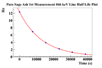
| + | The exponential decay plot is shown below | ||
| + | |||
| + | [[File:PureSageAsh 1stMeasurement 846keVHL ExpoPlot.png|200px]] | ||
| + | |||
| + | |||
| + | The fit parameters are | ||
| + | |||
| + | Constant: 2.50880 <math> \pm </math> 0.00287747 | ||
| + | |||
| + | Slope: -7.42478 <math> \pm </math> 0.0249932 <math> \times 10^{-5} </math> | ||
| + | |||
| + | Which yields a half life of 2.59 <math> \pm </math> 0.01 hours, which is within one standard deviation of Mn-56's half life (2.58 hours) | ||
| + | |||
| + | The lines that are characteristic with the highest branching ratios of Mn-56 (1810,2133 keV) are both present in the spectrum. This would lead me to believe it is indeed Mn-56 which is produced by either a proton knockout of Fe-57, or neutron capture on Mn-55. | ||
| + | |||
| + | There is also an 834 keV line present, but due to the long half life of Mn-54, this will take some time to analyze, but remember it is there! | ||
| + | |||
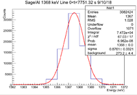
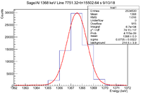
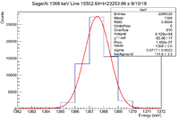
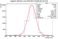
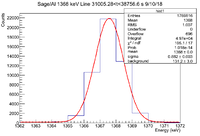
| + | ==1367.5 keV Line Analysis== | ||
| + | There is a line decaying at 1367.5 keV. Let's do an analysis on it to see if the isotope can be identified. The window of analysis is [1362,1372] | ||
| + | |||
| + | |||
| + | {| border="3" cellpadding="5" cellspacing="0" | ||
| + | || || 0<t<7751.32 s || 7751.32<t<15502.64 s || 15502.64<t<23253.96 s || 23253.96<t<31005.28 s || 31005.28<t<38756.6 s || 38756.6<t<46507.9 s | ||
| + | |- | ||
| + | || Histogram || [[File:LB SageAl 1368keV 0 t 7751 9 10 18.png|200px]] || [[File:LB SageAl 1368keV 7751 t 15502 9 10 18.png|200px]] || [[File:LB SageAl 1368keV 15502 t 23253 9 10 18.png|200px]] || [[File:LB SageAl 1368keV 23253 t 31005 9 10 18.png|200px]] || [[File:LB SageAl 1368keV 31005 t 38756 9 10 18.png|200px]] || [[File:LB SageAl 1368keV 38756 t 46507 9 10 18.png|200px]] | ||
| + | |- | ||
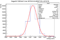
| + | ||Signal in Window || <math> 7.472 \times 10^4 </math> || <math> 6.7 \times 10^4 </math> || <math> 6.129 \times 10^4 </math> || <math> 5.567 \times 10^4 </math> || <math> 4.97 \times 10^4 </math> || <math> 4.525 \times 10^4 </math> | ||
| + | |- | ||
| + | ||Integrated Background || 2732 <math> \pm </math> 44 || 2145 <math> \pm </math> 39 || 1746 <math> \pm </math> 35 || 1552 <math> \pm </math> 33 || 1312 <math> \pm </math> 30 || 1188 <math> \pm </math> 29 | ||
| + | |- | ||
| + | ||Signal - Background || 71988 <math> \pm </math> 276.868 || 64855 <math> \pm </math> 261.765 || 59544 <math> \pm </math> 250.03 || 54118 <math> \pm </math> 238.241 || 48388 <math> \pm </math> 224.944 || 44062 <math> \pm </math> 214.688 | ||
| + | |- | ||
| + | ||Runtime (s) || 7751.32 || 7751.32 || 7751.32 || 7751.32 || 7751.32 || 7751.3 | ||
| + | |- | ||
| + | ||Rate (Hz) || 9.29 <math> \pm </math> 0.04 || 8.37 <math> \pm </math> 0.03 || 7.68 <math> \pm </math> 0.03 || 6.98 <math> \pm </math> 0.03 || 6.24 <math> \pm </math> 0.03 || 5.68 <math> \pm </math> 0.03 || | ||
| + | |- | ||
| + | |} | ||
| + | |||
| + | [[File:LB SageAL 1368keV HalfLifePlot.png|200px]] | ||
| + | |||
| + | The fit parameters are | ||
| + | |||
| + | constant: 2.22835e+00 +/- 2.95795e-03 | ||
| + | |||
| + | slope: -1.26126e-05 +/- 1.41004e-07 | ||
| + | |||
| + | which gives a half life of 15.26 +/- 0.17 hours. This is within 2 standard deviations of Na-24's half life. This isotope also has a line present at 2754 keV, which is present in the energy spectrum. Also this is the only isotope with branching ratios compatible with the gamma spectrum data. This would be a neutron capture on stable Na-23. | ||
| + | |||
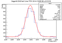
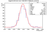
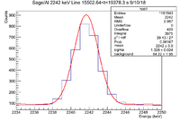
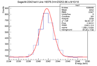
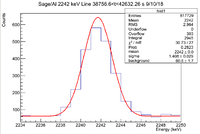
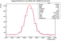
| + | ==2242 keV Analysis== | ||
| + | There is a decaying line seen at 2242 keV. The analysis was done in a 16 channel window from [2234,2250] | ||
| + | |||
| + | {| border="3" cellpadding="5" cellspacing="0" | ||
| + | || || 0<t<3875.66 s || 3875.66<t<7751.32 s || 7751.32<t<11626.98 s || 11626.98<t<15502.64 s || 15502.64<t<19378.3 s || 19378.3<t<23253.96 s || 23253.96<t<27129.62 s || 27129.62<t<31005.28 s || 31005.28<t<34880.94 s || 34880.94<t<38756.6 s || 38756.6<t<42632.26 s || 42632.26<t<46507.9 s | ||
| + | |||
| + | |- | ||
| + | || Histogram || [[File:LB SageAl 2242keVLine 0 t 3875.66 9 10 18.png|200px]] || [[File:LB SageAl 2242keVLine 3875.66 t 7751.32 9 10 18.png|200px]] || [[File:LB SageAl 2242keVLine 7751 t 11626 9 10 18.png|200px]] || [[File:LB SageAl 2242keVLine 11626 t 15502 9 10 18.png|200px]] || [[File:LB SageAl 2242keVLine 15502 t 19378 9 10 18.png|200px]] || [[File:LB SageAl 2242keVLine 19378 t 23253 9 10 18.png|200px]] || [[File:LB SageAl 2242keVLine 23253 t 27129 9 10 18.png|200px]] || [[File:LB SageAl 2242keVLine 27129 t 31005 9 10 18.png|200px]] || [[File:LB SageAl 2242keVLine 31005 t 34880 9 10 18.png|200px]] || [[File:LB SageAl 2242keVLine 34880 t 38756 9 10 18.png|200px]] || [[File:LB SageAl 2242keVLine 38756 t 42632 9 10 18.png|200px]] || [[File:LB SageAl 2242keVLine 42632 t 46507 9 10 18.png|200px]] | ||
| + | |- | ||
| + | ||Signal in Window || 4792 || 4625 || 4355 || 4124 || 3975 || 3759 || 3498 || 3479 || 3280 || 3041 || 2945 || 2807 | ||
| + | |- | ||
| + | ||Integrated Background ||1686.4 <math> \pm </math> 35.2 || 1567.36 <math> \pm </math> 33.76 || 1418.56 <math> \pm </math> 32.32 || 1355.68 <math> \pm </math> 31.52 || 1347.52 <math> \pm </math> 31.2 || 1300 <math> \pm </math> 30.72 || 1152.48 <math> \pm </math> 29.12 || 1198.24 <math> \pm </math> 29.44 || 1111.36 <math> \pm </math> 28.48 || 1012.48 <math> \pm </math> 27.36 || 969.6 <math> \pm </math> 27.2 || 925.76 <math> \pm </math> 26.08 | ||
| + | |- | ||
| + | ||Signal - Background || 3105.6 <math> \pm </math> 77.66 || 3057.64 <math> \pm </math> 75.93 || 2936.44 <math> \pm </math> 73.48 || 2768.32 <math> \pm </math> 71.54 || 2627.48 <math> \pm </math> 70.35 || 2459 <math> \pm </math> 68.58 || 2345.52 <math> \pm </math> 65.92 || 2280.76 <math> \pm </math> 65.92 || 2168.64 <math> \pm </math> 63.96 || 2028.52 <math> \pm </math> 61.56 || 1975.4 <math> \pm </math> 60.70 || 1881.24 <math> \pm </math> 59.05 | ||
| + | |- | ||
| + | ||Runtime (s) || 3875.66 || 3875.66 || 3875.66 || 3875.66 || 3875.66 || 3875.66 || 3875.66 || 3875.66 || 3875.66 || 3875.66 || 3875.66 || 3875.64 | ||
| + | |- | ||
| + | ||Rate (Hz) || 0.80 <math> \pm </math> 0.02 || 0.79 <math> \pm </math> 0.02 || 0.76 <math> \pm </math> 0.02 || 0.71 <math> \pm </math> 0.02 || 0.68 <math> \pm </math> 0.02 || 0.63 <math> \pm </math> 0.02 || 0.61 <math> \pm </math> 0.02 || 0.59 <math> \pm </math> 0.02 || 0.56 <math> \pm </math> 0.02 || 0.52 <math> \pm </math> 0.02 || 0.51 <math> \pm </math> 0.02 || 0.48 <math> \pm </math> 0.02 | ||
| + | |- | ||
| + | |} | ||
| + | |||
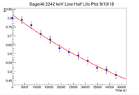
| + | [[File:LB 2242keVLine HLPlot.png|200px]] | ||
| + | |||
| + | The fit parameters are | ||
| + | |||
| + | Constant: -1.99924e-01 +/- 1.47295e-02 | ||
| + | |||
| + | Slope: -1.24500e-05 +/- 6.90105e-07 | ||
| + | |||
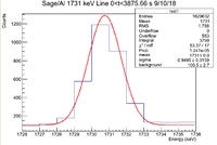
| + | ==1731 keV Analysis== | ||
| + | There is a decaying line seen at 1731 keV in the Sage/Al samples from 9/10/18. The analysis was done in a 10 channel window from [1726,1736] | ||
| + | |||
| + | {| border="3" cellpadding="5" cellspacing="0" | ||
| + | || || 0<t<3875.66 s || 3875.66<t<7751.32 s || 7751.32<t<11626.98 s || 11626.98<t<15502.64 s || 15502.64<t<19378.3 s || 19378.3<t<23253.96 s || 23253.96<t<27129.62 s || 27129.62<t<31005.28 s || 31005.28<t<34880.94 s || 34880.94<t<38756.6 s || 38756.6<t<42632.26 s || 42632.26<t<46507.9 s | ||
| + | |||
| + | |- | ||
| + | ||Histogram|| [[File:LB SageAl 1731keV 0 3875s 9 10 18.png|200px]] | ||
| + | |- | ||
| + | ||Signal in Window || 3799 || | ||
| + | |- | ||
| + | ||Integrated Background || 1005 +/- 27 | ||
| + | |- | ||
| + | ||Signal - Background || | ||
| + | |- | ||
| + | ||Runtime (s) || 3875.66 || 3875.66 || 3875.66 || 3875.66 || 3875.66 || 3875.66 || 3875.66 || 3875.66 || 3875.66 || 3875.66 || 3875.66 || 3875.64 | ||
| + | |- | ||
| + | ||Rate (Hz) || | ||
| + | |- | ||
| + | |} | ||
| + | |||
| + | =Production Optimization= | ||
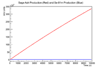
| + | The sage ash has a density of 0.1977 <math> \frac{g}{cm^3} </math>. To perform this I will use an 8 hour half life from the sage ash/Al sample irradiated on 9/10/18. | ||
| + | |||
| + | ==8 Hour Half Life (9/10/18)== | ||
| + | This section focuses on optimization for the sage/Al cylinder 8 hour half life performed above. The decay constant for that sample was -2.22732e-05 +/- 8.61118e-07 <math> s^{-1} </math>. The production rate is given by | ||
| + | |||
| + | <math> N(t) = \frac{n_T V_T}{\lambda} \int \sigma (E) \phi(E) dE (1-e^{- \lambda t}) </math> | ||
| + | |||
| + | For the sage ash, the cross section and the flux are unknown, so reduce this equation to | ||
| + | |||
| + | <math> N_{Sage/Al}(t) = \frac{d_T V_T}{\lambda}(1-e^{- \lambda t}) </math> | ||
| + | |||
| + | where <math> d_T </math> is the density of the target and <math> V_T </math> is the volume of the Al cylinder (assuming the cylinder will be completely filled with sage ash) | ||
| + | |||
| + | <math> V_T = 190.755 cm^3 </math> | ||
| + | |||
| + | |||
| + | For the selenium, we can compute the number of atoms per unit volume, <math> n_T </math>. The mass of a single selenium pellet is approximately 0.1g, while the atomic mass is 78.96u. So the number of atoms in a single selenium pellet is <math> 7.62 \times 10^{20} </math> atoms, which means | ||
| + | |||
| + | <math> n_{Se_T} = 3.812 \times 10^{22} \frac{atoms}{cm^3} </math> | ||
| + | |||
| + | Using the number of atoms vs. the density yields a highly unphysical result. Try using the density for the selenium as well. | ||
| + | |||
| + | <math> d_{Se_T} = 5 \frac{g}{cm^3} </math> | ||
| + | |||
| + | [[File:LB Se SageAsh ProdRate.png|200px]] | ||
| + | |||
| + | The capacitive decline and the differences in half life imply that the production rate will always be higher for the sage ash. | ||
| + | |||
| + | =NAA on Sage/Se Work= | ||
| + | The neutron capture cross sections can be found here https://inis.iaea.org/collection/NCLCollectionStore/_Public/28/060/28060364.pdf | ||
| + | |||
| + | Selenium cross sections begin at page 76. | ||
| + | |||
| + | To recreate the scenario for NAA (44 MeV, 46.34 degrees off of the beam axis), one possible reaction is Se80(N,g)Se81. This is essentially the reverse reaction from the PAA work. Note that Se-80 is more abundant than Se-82 (50% vs. 9%). Unfortunately there still is a chance of producing Se-79 (325000 year half life) through a neutron capture event on Se-78 which is 24% abundant. | ||
Latest revision as of 17:55, 8 November 2018
Mass Information
Note that only 2 samples were produced using the oven method (0.04% and 10%). The target masses are as follows
50% Se/Sage Sample
| Selenium Target (50% Sagebrush Se Mix) | Mass (g) |
| Outer Front Ni Foil | 0.6948 |
| Se Mass | 0.51 |
| Outer Se Mass | 0.1 |
| Sagebrush Leaves Mass | 0.4969 |
10% Sample
| Selenium Target (10% Sagebrush Se Mix) | Mass (g) |
| Outer Front Ni Foil | 0.2783 |
| Se Mass | 0.0523 |
| Outer Se Mass | 0.0971 |
| Sagebrush Leaves Mass | 0.5111 |
0.1% Se/Sage Sample
| Selenium Target (0.1% Sagebrush Se Mix) | Mass (g) |
| Outer Front Ni Foil | 1.1437 |
| Se Mass | 0.0559 |
| Outer Se Mass | 0.1118 |
| Sagebrush Leaves Mass | 50.1080 |
0.04% Sample
| Selenium Target (0.04% Sagebrush Se Mix) | Mass (g) |
| Outer Front Ni Foil | 0.5447 |
| Se Mass | 0.0020 |
| Outer Se Mass | 0.0992 |
| Sagebrush Leaves Mass | 4.9326 |
Time Cuts
The first step in the PAA process is to identify the time cuts used for the split run. This must be done for all samples (50%,10%,0.1%, and 0.04%).
50% Sage/Se Mixture Time Cuts
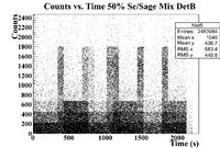
The 50% Se/Sage mixture was measure on Detector B (unshielded, so watch the SNR) on 5/24/17 for a total of 2130.540 seconds. The outer pure witness Se was measure first, and sub-run was roughly 300 seconds for the samples of interest, and 60 seconds for the Co-60 flag. The root command used to draw the timing information was
TTree* tree = MPA;
MPA->Draw("evt.Chan:evt.Sec>>hist2","evt.ADCid == 1");
which produced the histogram below
This seems a little sloppy, lets try a 1D histogram instead to see if the cuts are more clear
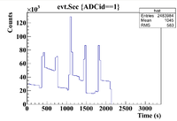
ROOT Command: MPA->Draw("evt.Sec>>hist","ADCid==1","");
This produced the histogram below
This seems much cleaner and clearly shows the time cuts
The time cuts are
0-300 (Pure Se)
375-440 (Co-60)
450-700 (Mixture)
715-780 (Co-60)
800-1010 (Pure Se)
1055-1150 (Co-60)
1160-1420 (Mixture)
1425-1495 (Co-60)
1500-1800 (Pure Se)
1810-1870 (Co-60)
1880-2100 (Mixture)
10% Sage/Se Mixture Time Cuts
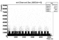
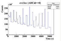
The 10% Se/Sage mixture was measured on Detector A (shielded) on 5/25/17 for a total of 5136.343 seconds. The mixture was measured first, and a sub-run was roughly 300 seconds for the Se samples and 60 seconds for the Co-60 flag. The root commands used were
TTree* tree = MPA;
MPA->Draw("evt.Chan:evt.Sec>>hist2","evt.ADCid == 0");
The time cut information is as follows
0-300 (Mixture)
300-360 (Co-60)
400-640 ( Pure Se)
680-710 (Co-60)
730-1020 (Mixture)
1030-1080 (Co-60)
1100-1360 ( Pure Se)
1400-1440 (Co-60)
1480-1775 (Mixture)
1800-1840 (Co-60)
1875-2150 (Pure Se)
2190-2220 (Co-60)
2250-2550 (Mixture)
2590-2620 (Co-60)
2650-2930 (Pure Se)
2950-3000 (Co-60)
3050-3300 (Mixture)
3390-3350 (Co-60)
3400-3690 (Pure Se)
3700-3750 (Co-60)
3775-4050 (Mixture)
4060-4100 (Co-60)
4120-4400 (Pure Se)
4420-4470 (Co-60)
4480-4770 (Mixture)
4790-4820 (Co-60)
4840-5130 (Pure Se)
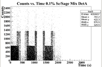
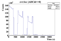
0.1% Sage/Se Mixture Time Cuts
The 0.1% Se/Sage mixture was measured on Detector A (shielded) on 5/24/17 for a total of 2130.540 seconds. The mixture was measured first, and a sub-run was roughly 300 seconds for the Se samples and 60 seconds for the Co-60 flag. The root commands used were
TTree* tree = MPA;
MPA->Draw("evt.Chan:evt.Sec>>hist2","evt.ADCid == 0");
which produced the histogram below
This seems a little sloppy, so let's repeat the procedure for the 50% sample
ROOT Command:ROOT Command: MPA->Draw("evt.Sec>>hist","ADCid==0","");
This produced the histogram below
This is again much better than the 2D histogram.
The time cuts are
0-300 (Mixture)
306-340 (Co-60)
376-640 (Pure Se)
650-720 (Co-60)
730-1010 (Mixture)
1020-1050 (Co-60)
1100-1350 (Pure Se)
1400-1460 (Co-60)
1470-1730 (Mixture)
1735-1800 (Co-60)
1804-2140 (Pure Se)
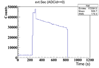
The histogram for the time cuts of the second run is shown below
The time cuts are
0-240 (Outer Se)
245-300 (Co-60)
305-820 (Mixture)
0.04% Sample Time Cuts
The 0.04% Se/Sage mixture was measured on Detector A (shielded) on 5/25/17 for a total of 1711.891 seconds. The mixture was measured first, and a sub-run was roughly 300 seconds for the Se samples and 60 seconds for the Co-60 flag. The root commands used were
TTree* tree = MPA;
MPA->Draw("evt.Sec>>hist2","evt.ADCid == 0");
The histogram representing the time cuts for the first run are shown below
The time cuts for this run are
0-290 (Mixture)
295-360 (Co-60)
370-684 (Pure Se)
The histogram representing the time cuts for the second run are shown below
The time cuts for this run are
0-300 (Mixture)
305-355 (Co-60)
360-650 (Pure Se)
660-735 (Co-60)
740-1020 (Mixture)
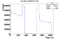
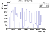
The histogram representing the time cuts for the third run are shown below
It would appear that first two time cuts are difficult to determine because the Co-60 flag's counts are on the same order as the sample's, so watch out for this next time! Each run should be roughly 300 seconds for the sample and 60 seconds for the Co-60 flag, so check the histograms to make sure there are no Co-60 lines to correct for this. To double check these time cuts I looked for Cl-34m in the mixture (which according to my 10% analysis was not present in the pure Se sample) and the Co-60 lines that may have overlapped. It seems there is a line near 1773 keV present in the mixture, but the 1332 keV line is missing in the mixture. Keep an eye out.
0-300 (Mixture,145 keV 1173 present | 1332 keV not present,good)
305-350 (Co-60, good)
360-650 (Pure Se, good)
660-710 (Co-60, good)
720-940 (Mixture, good)
1020-1070 (Co-60, good)
1100-1240 (Pure Se, good)
1270-1310 (Co-60, good)
1320-1630 (Mixture, good)
1660-1720 (Co-60, good)
1740-2030 (Pure Se, good)
2040-2120 (Co-60, good)
2130-2420 (Mixture, good)
2430-2490 (Co-60, good)
2500-2800 (Pure Se, good)
2810-2850 (Co-60, good)
2880-3150 (Mixture, good)
3170-3220 (Co-60, good)
3240-3510 (Pure Se, good)
3520-3580 (Co-60, good)
3600-3970 (Mixture, good)
4000-4060 (Co-60, good)
4100-4350 (Pure Se, good)
4370-4420 (Co-60, good)
4450-4710 (Mixture, good)
4730-4780 (Co-60, good)
4800-5080 (Pure Se, good)
5100-5160 (Co-60, good)
5190-5460 (Mixture)
5410-5600 (Co-60)
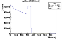
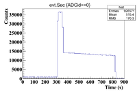
Below is the histogram representing the time cuts for the 4th run
Below are the time cuts
0-300 (Pure Se)
306-359 (Co-60)
362-818 (Mixture)
Gamma Spectrum Analysis
50% Sample Analysis
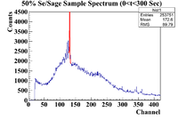
Below is the analysis table for the 50% Se/Sage mixture. The 103 keV line of Se-81m corresponds to a channel # of 130. Due to the sloppiness of the spectrum, I will use a linear + Gaussian fitting function and restrict my analysis to 6 channels because there are other energy lines nearby. Below is a sample spectrum for an idea of the resolution of Detector B for this measurement
As a comparison for the constant fit, here is a sample spectrum of the Se/Sage measured by Detector A
| 0<t<300 | ||
| Thin Window Histogram | ||
| Signal in Thin Window | ||
| Integrated Background | ||
| Signal - Background | ||
| Runtime (s) | ||
| Rate (Hz) | ||
| Integral Decay Correction (Hz) | ||
| Dead Time (%) | ||
| Dead Time Corrected Signal (Hz) | ||
| .Dat File Entry For HL Plot |
10% Sample Analysis
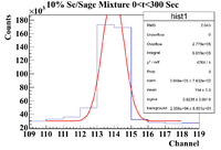
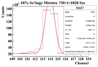
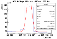
Below is the analysis table for the 10% Se/Sage mixture. The 103 keV line of Se-81m corresponds to a channel # of 113
Background and SNR Information
Below is a plot of the background in a 10 channel window around the short lived half life's energy peak of interest (103 keV). The long lived half live can be measured for at least a year even in a 0.1% by mass concentration, so it is less pressing. The values presented are weighted by the mass of the sage ash.
The fit parameters are
Constant: 4.50734e+00 +/- 2.42037e-03
Slope: -2.31438e-04 +/- 1.05610e-06
Which gives a rough half life of 49.92 +/- 0.23 minutes
Below is the SNR plotted in xmgrace
0.1% Sample Analysis
Below is the analysis table for the 0.1% Mixture, the 103 keV line for Se-81m corresponds to a channel # of 113.
0.04% Sample Analysis
Background and SNR Information
Below is the information for the background in the window [109,119] (Channel # here). The data was weighted by both the runtime and the mass of the sage ash.
The fit parameters here are
Constant: 3.42624e+00 +/- 3.71043e-03
Slope: -3.44115e-04 +/- 7.67333e-07
which gives a half life of 33.57 +/- 0.07 minutes.
The SNR plot is shown below
Fall 2018 Possible Sage Irradiation Activity Prediction
Isotope Search link: http://nucleardata.nuclear.lu.se/toi/
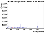
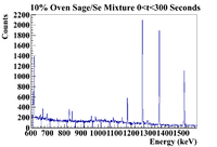
For this section I will attempt to identify the most active line within a sagebrush sample. The histograms that follow in this section will be weighted by the mass of the sage that was used for the sample. I will use the 10% Sage/Se mixture because it was processed using the oven method for dehydration. The mass was 0.5111g which gives a weighting factor of 1.9566 Below is a full spectrum for the time cut of 0 <t< 300 seconds.
It seems the two most prominent lines are around 150 keV and 250 keV, so let's try to study the decay of those first.
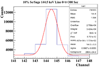
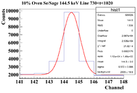
144.5 keV Line
Note: the x-axis for the first 2 histograms should be Energy (keV). This line is NOT present in the Pure Se Sample, so it should be a line produced by the sage itself.
Without any corrections, the half life here is 38.61 0.84 minutes. This is likely Cl-34m (32 min half life) produced by a (g,n) reaction on Cl-35 (75.76% natural abundance), which is stable, because a second line characteristic of Cl-34m was found (1176 keV). This could also be produced by a (g,pn) knockout on Ar-36 in air. This is chlorine since using the isotope search with an energy uncertainty of 5 keV and a half life uncertainty of 10 minutes, the only isotope that shared 146 and 1176 keV with branching ratios that made sense was Cl-34m.
9/10/18 Irradiation
The mass information is
Al Cylinder: 26.0249g
Sage Ash (oven method): 2.0913g
Beam off: 18:30
Calibration
Below is the runlist used for the calibration on Detector D
| Source | Serial No. | Reference Date | Activiy | Half life | Expected Energies (keV) | Line Seen (Channel No.) | Runtime (s) | Position | File Name | Date Measured |
| Mn-54 | J4-348 | 8/1/12 | 9.882 uCi | 312.20 days | 834.827 | 835.117 | 300.601 | 10 | LB_Mn_54_9_10_18_Pos10_DetD | 9/10/18 |
| Cs-137 | 129793 | 7/1/08 | 1.066 uCi | 30.08 years | 661.657 | 661.887 | 141.356 | 10 | LB_Cs137_9_10_18_Pos010_DetD | 9/10/18 |
| Co-60 | 129739 | 07/01/08 | 1.082 uCi | 1925.28 days | 1173.228, 1332.492 | 1173.338, 1332.564 | 232.521 | 10 | LB_Co60_9_10_18_Pos010_DetD | 9/10/18 |
| Ba-133 | 129790 | 07/01/08 | 1.188 uCi | 10.551 years | 80.9979, 276.3989, 302.8508, 356.0129, 383.8485 | 81.391, 276.741, 303.166, 356.315, 384.137 | 250.816 | 10 | LB_Ba133_9_10_18_Pos010_DetD | 9/10/18 |
The calibration coefficients are (according to my fits)
Intercept = -0.370972 +/- 0.616
Slope = 0.490352 +/- 0.000534241
The calibration used at the IAC was
Intercept = 0.272366
Slope = 0.490198
Efficiency
Below is a table of the runlist used for the efficiency on Detector D.
| Source | Serial No. | Reference Date | Activiy | Half life | Expected Energies (keV) | Start | Stop | Runtime (s) | Position | File Name | Date Measured |
| Mn-54 | J4-348 | 8/1/12 | 9.882 uCi | 312.20 days | 828.859 | 12:45 | 12:50 | 300.601 | 10 | LB_Mn_54_9_10_18_Pos10_DetD | 9/10/18 |
| Mn-54 | J4-348 | 8/1/12 | 9.882 uCi | 312.20 days | 828.859 | 12:52 | 12:57 | 305.787 | 20 | LB_Mn_54_9_10_Pos020_DetD | 9/10/18 |
| Mn-54 | J4-348 | 8/1/12 | 9.882 uCi | 312.20 days | 828.859 | 12:59:41 | 113:04 | 300.734 | 30 | LB_Mn_54_9_10_18_Pos030_DetD | 9/10/18 |
| Co-60 | 129740 | 07/01/08 | 10.42 uCi | 1925.28 days | 1173.228, 1332.492 | 18:17:35 | 18:24 | 409.011 | 80 | LB_Co60_9_10_18_Pos080_DetD | 9/10/18 |
| Co-60 | 129740 | 07/01/08 | 10.42 uCi | 1925.28 days | 1173.228, 1332.492 | 18:26:11 | 18:29 | 201.084 | 70 | LB_Co60_9_10_18_Pos070_DetD | 9/10/18 |
Runlist for 9/10/18 Irradiated Samples
| Sample | Date | Start | Stop | Runtime (s) | Position | Detector | % Dead | File Name |
| Sage Ash | 9/10/18 | 20:31:35 | 09:26 | 46507.875 | 40 | Detector D | < 2% | LB_SageAsh_OvenMethod_9_10_18_DetD_002 |
| Sage Ash | 9/11/18 | 14:59:50 | 10:57 | 71854.534 | 40 | Detector D | <1% | LB_SageAsh_OvenMethod_9_11_18_DetD_003 |
| Sage Ash | 9/12/18 | 11:01:05 | 89908.033 | 20 | Detector D | <1% | LB_SageAsh_OvenMethod_9_12_18_DetD_Pos20_001 | |
| Sage Ash | 9/13/18 | 12:03:02 | 73275.295 | 10 | Det D | <1% | LB_SageAsh_OvenMethod_9_13_18_DetD_Pos10_001 | |
| Sage Ash | 9/14/18 | 09:26:37 | 10:41 (9/17/18) | 10 | Det D | <1% | LB_SageAsh_OvenMethod_9_14_18_DetD_Pos10_001 | |
| Sage Ash | 9/17/18 | 10:51:02 | 10 | Det D | <1% | LB_SageAsh_OvenMethod_9_17_18_DetD_Pos10_001 | ||
| Sage Ash | 10/01/18 | 14:04:00 | Face of Detector | Det D | <1% | LB_SageAsh_OvenMethod_10_1_18_DetD_DetFace_002 |
September Sage+Al Analysis
https://wiki.iac.isu.edu/index.php/MCNP_Sim_of_Jack_Converter
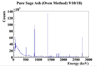
Below is the first measured histogram generated from the file LB_SageAsh_OvenMethod_9_10_18_DetD_002. Note that the Al cylinder and the sage ash were not separated, so there will be some lines from Al present. The histogram shown below is not weighted because there are two different samples in front of the detector at the same time (Al cylinder and sage ash). Once the lines have been identified, the mass will be taken into account
The command lines used in the directory /data/IAC/LB_Thesis_Analysis/Sept2018_SageAshBackground/Samples
.L Eff.C
Eff t
t.Loop(RangeMin,RangeMax);
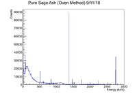
Below is a histogram of the second measurement taken overnight on 9/11/18
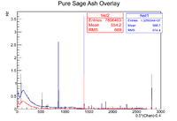
Now let's overlay these two histograms as a function of activity rather than counts to see if there are any lines that have decayed away that could possibly be identified. I did this as Hz vs. 0.5*(Chan)-0.4. The dithering proved to be quite difficult for both histograms.
Below is a table detailing the decaying/decayed lines. The relative rates were calculated using a linear fit plus a Gaussian fit, then the background subtracted activity was found.
| Line Seen (keV) | Isotope |
| 846 | Mn-56 |
| 1810 | Mn-56 |
| 2133 | Mn-56 |
| 1368 | Na-24 |
| 2754 | Na-24 |
Background Analysis
Below is the analysis of the background around the Se line of interest. The histograms were unweighted due to the presence of both the Al cylinder and the sage ash. The data points on the half life plot are weighted by the runtime. The energy window used was [90,130]. The times I concerned myself with spanned 5 half lives of Se (17184 sec) which were split cut into 10 different sets (runtime = 1718.4 sec).
The parameters are as follows
| 0<t<1718.4 s | 1718.4<t<3436.8 s | 3436.8<t<5155.2 s | 5155.2<t<6873.6 s | 6873.6<t<8592 s | 8592<t<10310.4 s | 10310.4<t<12028.8 s | 12028.8<t<13747.2 s | 13747.2<t<15461.6 s | 15461.6<t<17180 s | |
| Slope () | 5.853 0.562 | 5.33 0.54 | 4.981 0.532 | 5.423 0.521 | 6.234 0.511 | 5.155 0.503 | 4.703 0.496 | 4.053 0.489 | 4.49 0.49 | 4.506 0.503 |
| Intercept ( ) | 1051 61.9 | 998.8 59.6 | 974.6 58.7 | 871.7 57.4 | 731.4 56.2 | 796.7 55.4 | 807.3 54.6 | 841 53.9 | 836.8 54.5 | 868.6 55.4 |
| Integral from [90,130] | 39.45 2.04 | 36.90 1.96 | 35.44 1.92 | 34.18 1.89 | 32.99 1.85 | 31.74 1.82 | 30.83 1.80 | 29.95 1.77 | 30.98 1.78 | 31.76 1.82 |
Now the total background was found by integrating the linear fit function across the region of interest, in other words
To find the error in the integral, use the standard error propagation method
Since the partial derivatives are not taken with respect to the variable of integration and the function is analytic within the region, the derivative may be moved inside the integral. This action yields
Below is the initial plot of the background in the region from [90,130]
This plot has some outliers and fluctuations in the background that could be due to the presence of other sources (Dr. Dale was measuring very hot gallium on Det A during my overnight measurement).
10 Channel Analysis
The fits were done in a larger window [90,130] to get enough bins for a good fit, so I should be able to simply change the bounds of the integration to make the correction. There is definitely some randomness within the time cuts which produce bins with data above and below the fit line, which makes this more difficult. With the dithering, the peak on Detector A has a mean value of 103.949 kev, so the window I will analyze on Detector D (calibrated to energy) will be [99,109] keV
| 0<t<1718.4 s | 1718.4<t<3436.8 s | 3436.8<t<5155.2 s | 5155.2<t<6873.6 s | 6873.6<t<8592 s | 8592<t<10310.4 s | 10310.4<t<12028.8 s | 12028.8<t<13747.2 s | 13747.2<t<15461.6 s | 15461.6<t<17184 s | 17184 <t< 18902.4 s | 18902.4 <t< 20620.8 s | 20620.8<t<22339.2 s | 22339.2<t<24057.6 s | 24057.6<t<25776 s | 25776<t<27494.4 s | 27494.4<t<29212.8 s | 29212.8 <t< 30931.2 s | 30931.2 <t< 32649.6 s | 32649.6<t<34368 s | 34368<t<36086.4 s | 36086.4<t<37804.8 | 37804.8 <t< 39523.2 | 39523.2<t<41241.6 s | 41241.6 <t< 42960 s | 42960<t<44678.4 s | 44678.4 <t< 46396.8 s | |
| Slope () | 5.853 0.562 | 5.33 0.54 | 4.981 0.532 | 5.423 0.521 | 6.234 0.511 | 5.155 0.503 | 4.703 0.496 | 4.053 0.489 | 4.49 0.49 | 4.506 0.503 | 5.101 0.496 | 5.215 0.490 | 4.695 0.482 | 4.685 0.477 | 4.731 0.468 | 4.218 0.468 | 3.95 0.459 | 4.388 0.452 | 4.180 0.446 | 3.512 0.442 | 4.423 0.440 | 4.751 0.435 | 3.695 0.431 | 3.372 0.424 | 3.112 0.420 | 3.784 0.415 | 2.792 0.414 |
| Intercept ( ) | 1051 61.9 | 998.8 59.6 | 974.6 58.7 | 871.7 57.4 | 731.4 56.2 | 796.7 55.4 | 807.3 54.6 | 841 53.9 | 836.8 54.5 | 868.6 55.4 | 769.5 54.6 | 732.8 54.0 | 737.5 53.1 | 715.1 52.6 | 673.8 51.6 | 714.3 51.5 | 701.0 50.6 | 625.5 49.8 | 620.9 49.1 | 676.1 48.8 | 562.8 48.4 | 508.3 47.9 | 600.2 47.5 | 608 46.7 | 623 46.3 | 519.5 45.7 | 618.1 45.6 |
| Fit Function Integral from [99,109] | 9.67 0.50 | 9.04 0.48 | 8.69 0.47 | 8.35 0.46 | 8.03 0.45 | 7.76 0.44 | 7.54 0.44 | 7.35 0.43 | 7.59 0.43 | 7.78 0.44 | 7.57 0.44 | 7.42 0.43 | 7.13 0.42 | 7.00 0.42 | 6.78 0.41 | 6.71 0.41 | 6.47 0.40 | 6.30 0.40 | 6.14 0.39 | 6.06 0.39 | 5.95 0.39 | 5.83 0.38 | 5.73 0.38 | 5.58 0.37 | 5.51 0.37 | 5.31 0.37 | 5.29 0.36 |
| Stats Box Integral | 9943 | 9872 | 9699 | 9206 | 9110 | ||||||||||||||||||||||
| Stats Box Activity (Hz) | 9.58 0.07 | 9.12 0.07 | 8.76 0.07 | 6.74 0.06 | 8.15 0.07 | 7.80 0.07 | 7.60 0.07 | 7.53 0.07 | 7.75 0.07 | 7.84 0.07 | 7.64 0.07 | 7.54 0.07 | 7.20 0.06 | 6.97 0.06 | 6.95 0.06 | 6.79 0.06 | 6.60 0.06 | 6.41 0.06 | 6.31 0.06 | 6.19 0.06 | 6.09 0.06 | 5.98 0.06 | 5.79 0.06 | 5.74 0.06 | 5.64 0.06 | 5.36 0.06 | 5.30 0.06 |
| Corrected Background Measurement | 9.58 0.09 | 9.12 0.08 | 8.76 0.07 | 6.74 1.61 | 8.15 0.12 | 7.80 0.04 | 7.60 0.06 | 7.53 0.18 | 7.75 0.16 | 7.84 0.06 | 7.64 0.07 | 7.54 0.12 | 7.20 0.07 | 6.97 0.03 | 6.95 0.17 | 6.79 0.08 | 6.60 0.13 | 6.41 | 6.31 0.17 | 6.19 0.13 | 6.09 0.14 | 5.98 0.15 | 5.79 0.06 | 5.74 0.16 | 5.64 0.13 | 5.36 0.05 | 5.30 0.01 |
This looks like there are two separate half lives present, so split them up and fit.
The fit parameters for the first portion are
Slope: -2.22732e-05 +/- 8.61118e-07
Constant:2.25058e+00 +/- 6.19036e-03
Which gives a half life of 8.47 +/- 0.32 hours
The fit parameters for the second portion are
Constant: 2.24079e+00 +/- 5.78712e-03
Slope: -1.28411e-05 +/- 1.46816e-07
Which gives a half life of 14.99 +/- 0.17 hours
846 keV Line Analysis
Below is the analysis table. The energy window under study is [841,851]
The exponential decay plot is shown below
The fit parameters are
Constant: 2.50880 0.00287747
Slope: -7.42478 0.0249932
Which yields a half life of 2.59 0.01 hours, which is within one standard deviation of Mn-56's half life (2.58 hours)
The lines that are characteristic with the highest branching ratios of Mn-56 (1810,2133 keV) are both present in the spectrum. This would lead me to believe it is indeed Mn-56 which is produced by either a proton knockout of Fe-57, or neutron capture on Mn-55.
There is also an 834 keV line present, but due to the long half life of Mn-54, this will take some time to analyze, but remember it is there!
1367.5 keV Line Analysis
There is a line decaying at 1367.5 keV. Let's do an analysis on it to see if the isotope can be identified. The window of analysis is [1362,1372]
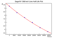
The fit parameters are
constant: 2.22835e+00 +/- 2.95795e-03
slope: -1.26126e-05 +/- 1.41004e-07
which gives a half life of 15.26 +/- 0.17 hours. This is within 2 standard deviations of Na-24's half life. This isotope also has a line present at 2754 keV, which is present in the energy spectrum. Also this is the only isotope with branching ratios compatible with the gamma spectrum data. This would be a neutron capture on stable Na-23.
2242 keV Analysis
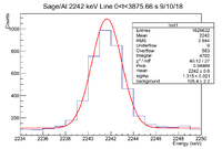
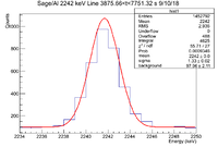
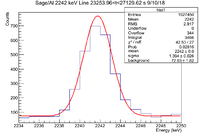
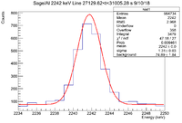
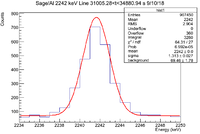
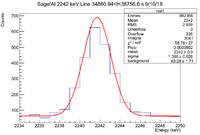
There is a decaying line seen at 2242 keV. The analysis was done in a 16 channel window from [2234,2250]
The fit parameters are
Constant: -1.99924e-01 +/- 1.47295e-02
Slope: -1.24500e-05 +/- 6.90105e-07
1731 keV Analysis
There is a decaying line seen at 1731 keV in the Sage/Al samples from 9/10/18. The analysis was done in a 10 channel window from [1726,1736]
Production Optimization
The sage ash has a density of 0.1977 . To perform this I will use an 8 hour half life from the sage ash/Al sample irradiated on 9/10/18.
8 Hour Half Life (9/10/18)
This section focuses on optimization for the sage/Al cylinder 8 hour half life performed above. The decay constant for that sample was -2.22732e-05 +/- 8.61118e-07 . The production rate is given by
For the sage ash, the cross section and the flux are unknown, so reduce this equation to
where is the density of the target and is the volume of the Al cylinder (assuming the cylinder will be completely filled with sage ash)
For the selenium, we can compute the number of atoms per unit volume, . The mass of a single selenium pellet is approximately 0.1g, while the atomic mass is 78.96u. So the number of atoms in a single selenium pellet is atoms, which means
Using the number of atoms vs. the density yields a highly unphysical result. Try using the density for the selenium as well.
The capacitive decline and the differences in half life imply that the production rate will always be higher for the sage ash.
NAA on Sage/Se Work
The neutron capture cross sections can be found here https://inis.iaea.org/collection/NCLCollectionStore/_Public/28/060/28060364.pdf
Selenium cross sections begin at page 76.
To recreate the scenario for NAA (44 MeV, 46.34 degrees off of the beam axis), one possible reaction is Se80(N,g)Se81. This is essentially the reverse reaction from the PAA work. Note that Se-80 is more abundant than Se-82 (50% vs. 9%). Unfortunately there still is a chance of producing Se-79 (325000 year half life) through a neutron capture event on Se-78 which is 24% abundant.
