|
|
| (5 intermediate revisions by the same user not shown) |
| Line 1: |
Line 1: |
| | + | |
| | + | <center><math> \underline{\textbf{Navigation} }</math> |
| | + | |
| | + | [[Uniform_distribution_in_Energy_and_Theta_LUND_files|<math>\vartriangleleft </math>]] |
| | + | [[VanWasshenova_Thesis#Moller_Scattering|<math>\triangle </math>]] |
| | + | [[Relativistic_Units|<math>\vartriangleright </math>]] |
| | + | |
| | + | </center> |
| | + | |
| | <pre>Total XSect=0.013866</pre> | | <pre>Total XSect=0.013866</pre> |
| | =97234 incident electrons= | | =97234 incident electrons= |
| Line 7: |
Line 16: |
| | | | |
| | | | |
| − | <center><math>t_{sim}(75nA)=\frac{N_{in}}{\frac{50E-9\ A}{}\frac{1\ C}{1\ A}\frac{}{1\ s}\frac{1\ e^{-}}{1.602E-19\ C}}=\frac{97234\ e^{-}}{468,164,794,007\ e^{-}/s}=2.07E-7\ s</math></center> | + | <center><math>t_{sim}(75nA)=\frac{N_{in}}{\frac{75E-9\ A}{}\frac{1\ C}{1\ A}\frac{}{1\ s}\frac{1\ e^{-}}{1.602E-19\ C}}=\frac{97234\ e^{-}}{468,164,794,007\ e^{-}/s}=2.07E-7\ s</math></center> |
| | | | |
| | | | |
| − | <center><math>t_{sim}(100nA)=\frac{N_{in}}{\frac{50E-9\ A}{}\frac{1\ C}{1\ A}\frac{}{1\ s}\frac{1\ e^{-}}{1.602E-19\ C}}=\frac{97234\ e^{-}}{624,219,725,343\ e^{-}/s}=1.56E-7\ s</math></center> | + | <center><math>t_{sim}(100nA)=\frac{N_{in}}{\frac{100E-9\ A}{}\frac{1\ C}{1\ A}\frac{}{1\ s}\frac{1\ e^{-}}{1.602E-19\ C}}=\frac{97234\ e^{-}}{624,219,725,343\ e^{-}/s}=1.56E-7\ s</math></center> |
| | | | |
| | | | |
| Line 48: |
Line 57: |
| | | | |
| | | | |
| − | <center>Occupancy(100nA)=<math>1.01926\%\frac{t_{sim}}{250E-9}</math></center> | + | <center>Occupancy=<math>1.01926\%\frac{t_{sim}}{250E-9}</math></center> |
| | | | |
| | | | |
| Line 56: |
Line 65: |
| | | | |
| | | | |
| − | <center><math>t_{sim}(75nA)=\frac{N_{in}}{\frac{50E-9\ A}{}\frac{1\ C}{1\ A}\frac{}{1\ s}\frac{1\ e^{-}}{1.602E-19\ C}}=\frac{N_{in}}{468,164,794,007\ e^{-}/s}=250E-9\ s\rightarrow N_{in}=117041.2\ e^{-}</math></center> | + | <center><math>t_{sim}(75nA)=\frac{N_{in}}{\frac{75E-9\ A}{}\frac{1\ C}{1\ A}\frac{}{1\ s}\frac{1\ e^{-}}{1.602E-19\ C}}=\frac{N_{in}}{468,164,794,007\ e^{-}/s}=250E-9\ s\rightarrow N_{in}=117041.2\ e^{-}</math></center> |
| | | | |
| | | | |
| − | <center><math>t_{sim}(100nA)=\frac{N_{in}}{\frac{50E-9\ A}{}\frac{1\ C}{1\ A}\frac{}{1\ s}\frac{1\ e^{-}}{1.602E-19\ C}}=\frac{N_{in}}{624,219,725,343\ e^{-}/s}=250E-9\ s\rightarrow N_{in}=156054.9\ e^{-}</math></center> | + | <center><math>t_{sim}(100nA)=\frac{N_{in}}{\frac{100E-9\ A}{}\frac{1\ C}{1\ A}\frac{}{1\ s}\frac{1\ e^{-}}{1.602E-19\ C}}=\frac{N_{in}}{624,219,725,343\ e^{-}/s}=250E-9\ s\rightarrow N_{in}=156054.9\ e^{-}</math></center> |
| | | | |
| | | | |
| − | Additionally, if we declare that every 2ns consists of a bunch of 1000 electrons each, then
| + | CEBAF has a bunch redition rate of 499MHz for hall B. For a current of 50nA, this implies: |
| | | | |
| − | <center><math>\frac{78027.5\ e^{-}}{\frac{1000\ e^{-}}{2E-9\ s}}=78.041\times 2E-9\ s=1.56E-7\ s</math></center> | + | <center><math>\frac{\frac{50E-9\ A}{}\frac{1C}{1A}\frac{}{1s}\frac{1\ e^{-}}{1.602E-19\ C}}{499E6\ Hz}=\frac{\frac{312,109,863,672\ e^{-}}{s}}{499E6\ Hz}=625\ e^{-}</math></center> |
| | | | |
| | | | |
| − | <center><math>\frac{117041.2\ e^{-}}{\frac{1000\ e^{-}}{2E-9\ s}}=117.041\times 2E-9\ s=2.34E-7\ s</math></center>
| + | If we declare that every 2ns consists of a bunch of 625 electrons each, then |
| | | | |
| | + | <center><math>\frac{78027.5\ e^{-}}{\left(\frac{625\ e^{-}}{2E-9\ s}\right)}=124.844\times 2E-9\ s=2.50E-7\ s</math></center> |
| | | | |
| − | <center><math>\frac{156054.9\ e^{-}}{\left(\frac{1000\ e^{-}}{2E-9\ s}\right)}=156.0549\times 2E-9\ s=3.12E-7\ s</math></center> | + | |
| | + | <center><math>\frac{117041.2\ e^{-}}{\left(\frac{625\ e^{-}}{2E-9\ s}\right)}=187.266\times 2E-9\ s=3.75E-7\ s</math></center> |
| | + | |
| | + | |
| | + | <center><math>\frac{156054.9\ e^{-}}{\left(\frac{625\ e^{-}}{2E-9\ s}\right)}=249.688\times 2E-9\ s=4.99E-7\ s</math></center> |
| | + | |
| | + | |
| | + | If we use these times as the times of simulation: |
| | + | |
| | + | |
| | + | <center>Occupancy(50nA)=<math>1.01926\%\frac{2.50E-7\ s}{250E-9}=1\%</math></center> |
| | + | |
| | + | |
| | + | <center>Occupancy(75nA)=<math>1.01926\%\frac{3.75E-7\ s}{250E-9}=1.5\%</math></center> |
| | + | |
| | + | |
| | + | <center>Occupancy(100nA)=<math>1.01926\%\frac{4.99E-7\ s}{250E-9}=2\%</math></center> |
| | | | |
| | ==Method 2== | | ==Method 2== |
| Line 94: |
Line 120: |
| | | | |
| | | | |
| − | <center>Occupancy(50nA)=<math>\frac{3698.7}{270}\frac{3.11E-7}{250E-9}\frac{1}{112}\frac{100}{12}=0.82\%</math></center> | + | <center>Occupancy(50nA)=<math>\frac{3698.7}{270}\frac{250E-9}{3.11E-7}\frac{1}{112}\frac{100}{12}=0.82\%</math></center> |
| | + | |
| | + | |
| | + | |
| | + | <center>Occupancy(75nA)=<math>\frac{3698.7}{270}\frac{250E-9}{2.07E-7}\frac{1}{112}\frac{100}{12}=1.23\%</math></center> |
| | + | |
| | + | |
| | + | |
| | + | <center>Occupancy(100nA)=<math>\frac{3698.7}{270}\frac{250E-9}{1.56E-7}\frac{1}{112}\frac{100}{12}=1.63\%</math></center> |
| | | | |
| | | | |
| | + | ---- |
| | | | |
| − | <center>Occupancy(75nA)=<math>\frac{3698.7}{270}\frac{2.07E-7}{250E-9}\frac{1}{112}\frac{100}{12}=1.23\%</math></center>
| |
| | | | |
| | + | <center><math> \underline{\textbf{Navigation} }</math> |
| | | | |
| | + | [[Uniform_distribution_in_Energy_and_Theta_LUND_files|<math>\vartriangleleft </math>]] |
| | + | [[VanWasshenova_Thesis#Moller_Scattering|<math>\triangle </math>]] |
| | + | [[Relativistic_Units|<math>\vartriangleright </math>]] |
| | | | |
| − | <center>Occupancy(100nA)=<math>\frac{3698.7}{270}\frac{1.56E-7}{250E-9}\frac{1}{112}\frac{100}{12}=1.63\%</math></center>
| + | </center> |
[math] \underline{\textbf{Navigation} }[/math]
[math]\vartriangleleft [/math]
[math]\triangle [/math]
[math]\vartriangleright [/math]
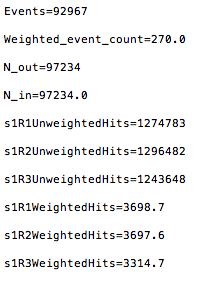
Total XSect=0.013866
97234 incident electrons
[math]t_{sim}(50nA)=\frac{N_{in}}{\frac{50E-9\ A}{}\frac{1\ C}{1\ A}\frac{}{1\ s}\frac{1\ e^{-}}{1.602E-19\ C}}=\frac{97234\ e^{-}}{312,109,862,672\ e^{-}/s}=3.11E-7\ s[/math]
[math]t_{sim}(75nA)=\frac{N_{in}}{\frac{75E-9\ A}{}\frac{1\ C}{1\ A}\frac{}{1\ s}\frac{1\ e^{-}}{1.602E-19\ C}}=\frac{97234\ e^{-}}{468,164,794,007\ e^{-}/s}=2.07E-7\ s[/math]
[math]t_{sim}(100nA)=\frac{N_{in}}{\frac{100E-9\ A}{}\frac{1\ C}{1\ A}\frac{}{1\ s}\frac{1\ e^{-}}{1.602E-19\ C}}=\frac{97234\ e^{-}}{624,219,725,343\ e^{-}/s}=1.56E-7\ s[/math]
Method 1
CLAS12 Occupancy[math]\equiv\frac{N_{hits}}{N_{evt}}\frac{t_{sim}}{\Delta t}\frac{1}{112}\frac{100}{12}[/math]
Using the unweighted amounts
Occupancy(50nA)=[math]\frac{1274783}{92967}\frac{3.11E-7}{250E-9}\frac{1}{112}\frac{100}{12}=1.27\%[/math]
Occupancy(75nA)=[math]\frac{1274783}{92967}\frac{2.07E-7}{250E-9}\frac{1}{112}\frac{100}{12}=0.844\%[/math]
Occupancy(100nA)=[math]\frac{1274783}{92967}\frac{1.56E-7}{250E-9}\frac{1}{112}\frac{100}{12}=0.637\%[/math]
Using the weighted amounts
Occupancy(50nA)=[math]\frac{3698.7}{270}\frac{3.11E-7}{250E-9}\frac{1}{112}\frac{100}{12}=1.27\%[/math]
Occupancy(75nA)=[math]\frac{3698.7}{270}\frac{2.07E-7}{250E-9}\frac{1}{112}\frac{100}{12}=0.844\%[/math]
Occupancy(100nA)=[math]\frac{3698.7}{270}\frac{1.56E-7}{250E-9}\frac{1}{112}\frac{100}{12}=0.637\%[/math]
The non-time terms can be considered to be constant since they are either simple number such as 12 or functions which depend on the same variables such as the number of hits and number of events (Both terms are found by [math]\sigma N_{in}\rho l[/math],thus are only multiples of each other). We can simplify this expression by:
Occupancy=[math]1.01926\%\frac{t_{sim}}{250E-9}[/math]
If 250ns is the time limit, then solving the time of simulation backwards will give the number of incident electrons within that window.
[math]t_{sim}(50nA)=\frac{N_{in}}{\frac{50E-9\ A}{}\frac{1\ C}{1\ A}\frac{}{1\ s}\frac{1\ e^{-}}{1.602E-19\ C}}=\frac{N_{in}}{312,109,862,672\ e^{-}/s}=250E-9\ s\rightarrow N_{in}=78027.5\ e^{-}[/math]
[math]t_{sim}(75nA)=\frac{N_{in}}{\frac{75E-9\ A}{}\frac{1\ C}{1\ A}\frac{}{1\ s}\frac{1\ e^{-}}{1.602E-19\ C}}=\frac{N_{in}}{468,164,794,007\ e^{-}/s}=250E-9\ s\rightarrow N_{in}=117041.2\ e^{-}[/math]
[math]t_{sim}(100nA)=\frac{N_{in}}{\frac{100E-9\ A}{}\frac{1\ C}{1\ A}\frac{}{1\ s}\frac{1\ e^{-}}{1.602E-19\ C}}=\frac{N_{in}}{624,219,725,343\ e^{-}/s}=250E-9\ s\rightarrow N_{in}=156054.9\ e^{-}[/math]
CEBAF has a bunch redition rate of 499MHz for hall B. For a current of 50nA, this implies:
[math]\frac{\frac{50E-9\ A}{}\frac{1C}{1A}\frac{}{1s}\frac{1\ e^{-}}{1.602E-19\ C}}{499E6\ Hz}=\frac{\frac{312,109,863,672\ e^{-}}{s}}{499E6\ Hz}=625\ e^{-}[/math]
If we declare that every 2ns consists of a bunch of 625 electrons each, then
[math]\frac{78027.5\ e^{-}}{\left(\frac{625\ e^{-}}{2E-9\ s}\right)}=124.844\times 2E-9\ s=2.50E-7\ s[/math]
[math]\frac{117041.2\ e^{-}}{\left(\frac{625\ e^{-}}{2E-9\ s}\right)}=187.266\times 2E-9\ s=3.75E-7\ s[/math]
[math]\frac{156054.9\ e^{-}}{\left(\frac{625\ e^{-}}{2E-9\ s}\right)}=249.688\times 2E-9\ s=4.99E-7\ s[/math]
If we use these times as the times of simulation:
Occupancy(50nA)=[math]1.01926\%\frac{2.50E-7\ s}{250E-9}=1\%[/math]
Occupancy(75nA)=[math]1.01926\%\frac{3.75E-7\ s}{250E-9}=1.5\%[/math]
Occupancy(100nA)=[math]1.01926\%\frac{4.99E-7\ s}{250E-9}=2\%[/math]
Method 2
CLAS12 Occupancy[math]\equiv\frac{N_{hits}}{N_{evt}}\frac{\Delta t}{t_{sim}}\frac{1}{112}\frac{100}{12}[/math]
Using the unweighted amounts
Occupancy(50nA)=[math]\frac{1274783}{92967}\frac{250E-9}{3.11E-7}\frac{1}{112}\frac{100}{12}=0.82\%[/math]
Occupancy(75nA)=[math]\frac{1274783}{92967}\frac{250E-9}{2.07E-7}\frac{1}{112}\frac{100}{12}=1.23\%[/math]
Occupancy(100nA)=[math]\frac{1274783}{92967}\frac{250E-9}{1.56E-7}\frac{1}{112}\frac{100}{12}=1.63\%[/math]
Using the weighted amounts
Occupancy(50nA)=[math]\frac{3698.7}{270}\frac{250E-9}{3.11E-7}\frac{1}{112}\frac{100}{12}=0.82\%[/math]
Occupancy(75nA)=[math]\frac{3698.7}{270}\frac{250E-9}{2.07E-7}\frac{1}{112}\frac{100}{12}=1.23\%[/math]
Occupancy(100nA)=[math]\frac{3698.7}{270}\frac{250E-9}{1.56E-7}\frac{1}{112}\frac{100}{12}=1.63\%[/math]
[math] \underline{\textbf{Navigation} }[/math]
[math]\vartriangleleft [/math]
[math]\triangle [/math]
[math]\vartriangleright [/math]
