Difference between revisions of "LB RunGroupC Vertex"
| (610 intermediate revisions by 2 users not shown) | |||
| Line 1: | Line 1: | ||
Vertex Reconstruction studies | Vertex Reconstruction studies | ||
| − | = | + | =Inclusive electron GEMC 2.4 & Coatjava 2.4= |
| − | + | [[LB_GEMC2.4CJ2.4_Vertex]] | |
| − | [[ | + | [[Phi angle gcard vs. LUND]] |
| − | |||
| − | |||
| − | + | ==Summary== | |
| + | |||
| + | Set all histogram ranges to -6,6 cm and bin sizes of 0.1 cm | ||
| + | |||
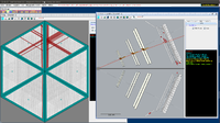
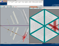
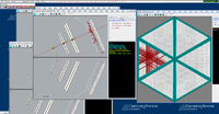
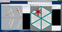
| + | Below are some of the sample GEMC simulations as seen in the CED | ||
| + | |||
| + | |||
| + | {|border="5" | ||
| + | || 6cm Z Target, No Rotation || 6cm Z Target, 270 Degree Rotation || 6cm Z Target, 90 Degree Rotation || 2cm Y Target, 30 Degree Rotation || 2cm Y Target, 180 Degree Rotation || 2cm X Target, 90 Degree Rotation || 2cm X Target, 270 Degree Rotation | ||
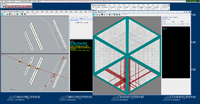
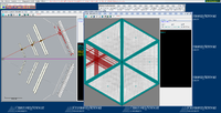
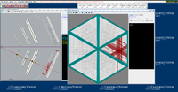
| + | |- | ||
| + | || [[File:Ced ZRaster 0DegRot.png|200px]] || [[File:6cm ZTarg 270DegRot CED.png|200px]] || [[File:Ced ZRaster 90DegRot.png|200px]] || [[File:2cm YRaster 30DegRot ced.png|200px]] || [[File:Ced YRaster 180DegRot.png|200px]] || [[File:Ced XRaster 90DegRot.png|200px]] || [[File:Ced XRaster 270DegRot.png|200px]] | ||
| + | |- | ||
| + | |}<br> | ||
| + | |||
| + | There is a bash script on lds2 that will create Vx,Vy, and Vz differences for a point target, 3 2 cm line targets (in X,Y, and Z), 2 2D targets (one XZ target where X = 2cm and Z = 6cm and another where Y = 2cm and Z = 6 cm), and one 3D target where X = Y = 2cm and Z = 6cm. A 6 GeV electron is fired at angles <math>\theta = 25</math> degrees and <math>\phi = 30</math> degrees. The path to the script is /home/lds/src/CLAS/GEMC/experiments/eg12/vertex and the file is called run.exe. To run it you must be in a tcsh and have the setup in the GEMC directory sourced. Then simply hit ./run.exe. Right now the number of events is small (100), but that can easily be changed within the script. | ||
| + | |||
| + | ===Point target X,Y,Z=0 cm=== | ||
| + | |||
| + | |||
| + | |||
| + | The histograms below are using a 6 GeV electron fired at an angles of 25 degrees in theta and 0 degrees in phi. | ||
| + | |||
| + | For the plots below, I used the following gcard, sample LUND file, and commands in GEMC 2.4, coat-java 2.4, and ROOT | ||
| + | |||
| + | gcard: | ||
<gcard> | <gcard> | ||
<detector name="../../../../clas12/fc/forwardCarriage" factory="TEXT" variation="original"/> | <detector name="../../../../clas12/fc/forwardCarriage" factory="TEXT" variation="original"/> | ||
| − | <detector name="../../../../clas12/dc/dc" factory="TEXT" variation=" | + | <detector name="../../../../clas12/dc/dc" factory="TEXT" variation="ccdb"/> |
<detector name="../../../../clas12/ec/ec" factory="TEXT" variation="original"/> | <detector name="../../../../clas12/ec/ec" factory="TEXT" variation="original"/> | ||
<detector name="../../../../clas12/ctof/ctof" factory="TEXT" variation="original"/> | <detector name="../../../../clas12/ctof/ctof" factory="TEXT" variation="original"/> | ||
| − | <detector name="../../../../clas12/ftof/ftof" factory="TEXT" variation=" | + | <detector name="../../../../clas12/ftof/ftof" factory="TEXT" variation="java"/> |
<detector name="../../../../clas12/htcc/htcc" factory="TEXT" variation="original"/> | <detector name="../../../../clas12/htcc/htcc" factory="TEXT" variation="original"/> | ||
<detector name="../../../../clas12/pcal/pcal" factory="TEXT" variation="javageom"/> | <detector name="../../../../clas12/pcal/pcal" factory="TEXT" variation="javageom"/> | ||
| + | <detector name="../../../../clas12/magnets/solenoid" factory="TEXT" variation="original"/> | ||
<option name="SCALE_FIELD" value="clas12-torus-big, -1"/> | <option name="SCALE_FIELD" value="clas12-torus-big, -1"/> | ||
| − | + | <option name="HALL_FIELD" value="clas12-solenoid"/> | |
| − | + | <option name="OUTPUT" value="evio,eg12_sol_75k_No_Raster.ev"/> | |
| − | |||
</gcard> | </gcard> | ||
| − | + | Sample LUND File: | |
| + | |||
| + | 1 1 1 1 1 1.00029 0.0718059 0.937771 1.48222 0.789865 | ||
| + | 1 -1 1 11 0 0 0 2.53564 5.43788 6 0.000511 0 0 0 | ||
| + | 1 1 1 1 1 1.00029 0.0718059 0.937771 1.48222 0.789865 | ||
| + | 1 -1 1 11 0 0 0 2.53564 5.43788 6 0.000511 0 0 0 | ||
| + | 1 1 1 1 1 1.00029 0.0718059 0.937771 1.48222 0.789865 | ||
| + | 1 -1 1 11 0 0 0 2.53564 5.43788 6 0.000511 0 0 0 | ||
| + | |||
| + | |||
| + | GEMC Command: | ||
| + | |||
| + | ~/src/CLAS/GEMC/source/gemc -USE_GUI=0 -INPUT_GEN_FILE="LUND,No_Raster.LUND" -N=75000 eg12_sol_No_Raster.gcard | ||
| + | |||
| + | Coat-Java 2.4 command: | ||
| + | |||
| + | ~/src/CLAS/coatjava-2.4/bin/clas12-reconstruction -i ../files/vertex/vertex.evio -config GEOM::new=true -config MAG::torus=-1.0 -config MAG::solenoid=1.0 -o ../files/vertex/vertex_rec.evio -s DCHB:DCTB:EC:FTOF:EB -config DATA::mc=true -config DCTB::useRaster=true | ||
| + | |||
| + | Sample ROOT command: | ||
| + | |||
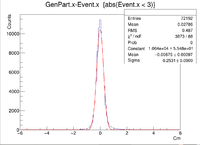
| + | clas12->Draw("GenPart.x - Event.x","abs(Event.x)<3"); | ||
| + | |||
| + | |||
| + | {|border="5" | ||
| + | ! || No Rastering | ||
| + | |- | ||
| + | || Vx Difference || [[File:NoRaster VxDifference sol.png|200px]] | ||
| + | |- | ||
| + | || Vy Difference || [[File:NoRaster VyDifference sol.png|200px]] | ||
| + | |- | ||
| + | || Vz Difference || [[File:NoRaster VzDifference sol.png|200px]] | ||
| + | |- | ||
| + | || X Resolution (cm) || 0.2362 +/- 0.0008 | ||
| + | |- | ||
| + | ||Y Resolution(cm) || 0.09809 +/- 0.00033 | ||
| + | |- | ||
| + | ||Z Resolution (cm) || 0.05435 +/- 0.00017 | ||
| + | |}<br> | ||
| + | |||
| + | These histograms raise some questions. To begin I created a LUND file with 6 GeV incident electrons at 25 degrees in theta and 0 degrees in phi. All of the vertex positions were set to 0. I then ran GEMC 2.4 using the command line | ||
| + | ~/src/CLAS/GEMC/source/gemc -USE_GUI=0 -INPUT_GEN_FILE="LUND,No_Raster.LUND" -N=75000 eg12_sol_No_Raster.gcard | ||
| + | |||
| + | which created an output file called eg12_sol_75k_No_Raster.ev. After that the reconstruction command line used was | ||
| + | |||
| + | ~/src/CLAS/coatjava-2.4/bin/clas12-reconstruction -i eg12_sol_75k_No_Raster.ev-config GEOM::new=true -config MAG::torus=-1.0 -config MAG::solenoid=1.0 -o eg12_sol_75k_No_Raster_rec.evio -s DCHB:DCTB:EC:FTOF:EB -config DATA::mc=true -config DCTB::useRaster=true | ||
| + | |||
| + | After the reconstruction a root file was created using | ||
| + | |||
| + | ~/src/CLAS/evio2root/bin/evio2root eg12_sol_75k_No_Raster_rec.evio eg12_sol_75k_No_Raster_rec.root 75000 | ||
| + | |||
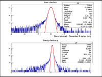
| + | A plot was then created to show the X Vertex and Y Vertex Differences | ||
| + | |||
| + | [[File:NoRaster Vx YDifference.png|200px]] | ||
| + | |||
| + | The first question is why is there a shift in the Y Difference. What would make X more centered around 0? The next question is when rastering begins, why do the resolutions in the X Vertices remain unchanged while the resolutions in the Y Vertices change? | ||
| + | |||
| + | ===Point in 2-D but extended target in 1-D=== | ||
| + | |||
| + | Two vertex variables are fixed at zero and the third vertex variable is altered. A 6 GeV electron was fired at angles of 25 degrees in theta and 0 degrees in phi. | ||
| + | |||
| + | The gcard used had the same detector parts as above, but the filename and pathways were changed. | ||
| + | |||
| + | Below is a sample line from the LUND files: | ||
| + | |||
| + | For 2cm X Target: 1 1 1 1 1 1.00029 0.0718059 0.937771 1.48222 0.789865 | ||
| + | 1 -1 1 11 0 0 0 2.53564 5.43788 6 0.000511 0.999484 0 0 | ||
| + | |||
| + | For 2cm Y Target: 1 1 1 1 1 1.00029 0.0718059 0.937771 1.48222 0.789865 | ||
| + | 1 -1 1 11 0 0 0 2.53564 5.43788 6 0.000511 0 0.999484 0 | ||
| + | |||
| + | For 2cm Z Target: 1 1 1 1 1 1.00029 0.0718059 0.937771 1.48222 0.789865 | ||
| + | 1 -1 1 11 0 0 0 2.53564 5.43788 6 0.000511 0 0 2.99845 | ||
| + | |||
| + | |||
| + | Also, here are the GEMC, Coat-Java, and a sample ROOT command. | ||
| + | |||
| + | GEMC: ~/src/CLAS/GEMC/source/gemc -USE_GUI=0 -INPUT_GEN_FILE="LUND,test.LUND" -N=100 eg12.gcard | ||
| + | |||
| + | Coat-Java:~/src/CLAS/coatjava-2.4/bin/clas12-reconstruction -i ../files/vertex/vertex.evio -config GEOM::new=true -config MAG::torus=-1.0 -config MAG::solenoid=1.0 -o ../files/vertex/vertex_rec.evio -s DCHB:DCTB:EC:FTOF:EB -config DATA::mc=true -config DCTB::useRaster=true | ||
| + | |||
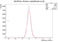
| + | Sample ROOT command: clas12->Draw("GenPart.x - Event.x","abs(Event.x)<2"); | ||
| + | |||
| + | {|border="5" | ||
| + | ! || 2cm X Raster, Y=0,Z=0 || 2 cm Y Raster, X=0,Z=0|| 2 cm Z Raster ,X=0,Y=0|| 6 cm Z Raster ,X=0,Y=0 | ||
| + | |- | ||
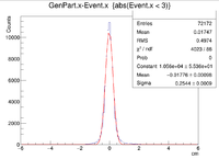
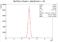
| + | || Vx Difference || [[File:1cm XRaster VxDifference sol 75k.png|200px]] || [[File:1cm YRaster VxDifference sol.png|200px]] || [[File:2cm ZRaster VxDifference sol.png|200px]] || [[File:3cm ZRaster VxDifference sol.png|200px]] | ||
| + | |- | ||
| + | || Vy Difference || [[ File:1cm XRaster VyDifference sol.png|200px]] || [[File:YRaster Eventy.png |200px]] || [[File:2cm ZRaster VyDifference sol.png|200px]] || [[File:3cm ZRaster VyDifference sol.png|200px]] | ||
| + | |- | ||
| + | || Vz Difference || [[ File:1cm XRaster VzDifference sol.png|200px]] || [[ File:1cm YRaster VzDifference sol.png|200px]] || [[File:2cm ZRaster VzDifference.png|200px]] || [[File:3cm ZRaster VZDifference sol 75k.png|200px]] | ||
| + | |- | ||
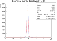
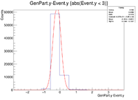
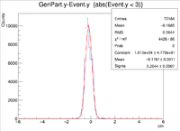
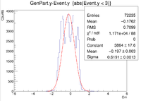
| + | || X Resolution (cm) || 0.2658 +/- 0.0010 || 0.2531 +/- 0.0009 || 0.2544 +/- 0.0009 || 0.2539 +/- 0.0009 | ||
| + | |- | ||
| + | ||Y Resolution(cm) || 0.1728 +/- 0.0007 || 0.2368 +/- 0.0007 || 0.2644 +/- 0.0007 || 0.6191 +/- 0.0013 | ||
| + | |- | ||
| + | ||Z Resolution (cm) || 0.1792 +/- 0.0006 || 0.1998 +/- 0.0004 || 0.4318 +/- 0.0009 || 1.105 +/- 0.002 | ||
| + | |}<br> | ||
| + | |||
| + | === Extended target -3 < Z < 3 cm === | ||
| + | |||
| + | For the plots below a 6 GeV electron was fired at angles theta = 25 degrees and phi = 0 degrees. There were 3 separate simulations ran for when -3 cm < Z < 3 cm. The first was a 2-D target with -3 cm < Z < 3 cm and -1 cm < X < 1 cm and Y = 0 cm, while the second had the same values for Z, but instead -1 cm < Y < 1cm and X = 0 cm. The final set of plots was created using -3 cm < Z < 3 cm , -1 cm < X < 1 cm, and -1 cm < Y < 1 cm. | ||
| + | |||
| + | Below are some of the sample LUND files used. | ||
| + | |||
| + | For the XZ Target: | ||
| + | |||
| + | 1 1 1 1 1 1.00029 0.0718059 0.937771 1.48222 0.789865 | ||
| + | 1 -1 1 11 0 0 0 2.53564 5.43788 6 0.000511 -0.67418 0 2.99845 | ||
| + | 1 1 1 1 1 1.00029 0.0718059 0.937771 1.48222 0.789865 | ||
| + | 1 -1 1 11 0 0 0 2.53564 5.43788 6 0.000511 0.894402 0 -1.30429 | ||
| + | |||
| + | For the YZ Target: | ||
| + | |||
| + | 1 1 1 1 1 1.00029 0.0718059 0.937771 1.48222 0.789865 | ||
| + | 1 -1 1 11 0 0 0 2.53564 5.43788 6 0.000511 0 -0.67418 2.99845 | ||
| + | 1 1 1 1 1 1.00029 0.0718059 0.937771 1.48222 0.789865 | ||
| + | 1 -1 1 11 0 0 0 2.53564 5.43788 6 0.000511 0 0.894402 -1.30429 | ||
| + | |||
| + | |||
| + | For the XYZ Target: | ||
| + | |||
| + | 1 1 1 1 1 1.00029 0.0718059 0.937771 1.48222 0.789865 | ||
| + | 1 -1 1 11 0 0 0 2.53564 5.43788 6 0.000511 -0.67418 -0.434764 2.99845 | ||
| + | 1 1 1 1 1 1.00029 0.0718059 0.937771 1.48222 0.789865 | ||
| + | 1 -1 1 11 0 0 0 2.53564 5.43788 6 0.000511 -0.536687 -0.0300528 2.68321 | ||
| + | 1 1 1 1 1 1.00029 0.0718059 0.937771 1.48222 0.789865 | ||
| + | 1 -1 1 11 0 0 0 2.53564 5.43788 6 0.000511 0.488611 0.0800873 2.74486 | ||
| + | |||
| + | |||
| + | The GEMC and Coat-Java command lines are similar to the previously seen commands. The only things that changed were the LUND file names, and the ev/evio filenames. The command lines can be seen at the top of the histograms. | ||
| + | |||
| + | [[VertREC_9-22-16_table_3ltZgt-3]] | ||
| + | |||
| + | === Extended target in Z. Vy shift analysis === | ||
| + | |||
| + | All Histograms below were created by simply making the target longer along the Z axis. Each case uses vertex points for X and Y ranging from -1cm to 1cm | ||
| + | |||
| + | [[VertREC_9-22-16_table_3ltZgt-3_1gtRlt-1]] | ||
| + | |||
| + | === Localized Vertex Resolution Investigation of Line Targets === | ||
| + | |||
| + | GEMC was ran to create electrons being produced in a line along certain axes. These include three separate 2cm targets centered at (0,0,0) in the X, Y , and Z directions. The final target is a line along the Z axis centered at (0,0,0) that is 6cm long. The generated electrons were shot at 25 degrees in theta and 0 degrees in phi at an energy of 6GeV. | ||
| + | |||
| + | Here is an example of how the cuts were made. Consider the case of a 2cm line target in the Z direction centered at (0,0,0). Closed intervals begin at the end of the target and are 0.1cm long. So the first interval would be [-1.0,-0.9], then the next would be [-0.9, -0.8] and so on until the entire target is covered. The events in the EVENTHB bank were cut so that in any given interval there would be a margin of +/- 1cm from the end of the area of interest to remove any outliers that may cause the histograms to have long tails. | ||
| + | |||
| + | |||
| + | |||
| + | |||
| + | Below are the histograms for the 2cm line target in Y,X=0,Z=0. The electrons were fired with an energy of 6 GeV at 25 degrees in theta at 0 degrees in phi. | ||
| + | |||
| + | [[2cm YLineTarg 0 Degree Rotation 09/23/16]] | ||
| + | |||
| + | Below are the histograms for a 2cm target along the Y axis, X = 0 Z = 0. The electrons were fired with an energy of 6 GeV at 25 degrees in theta and 180 degrees in phi. | ||
| + | |||
| + | [[2cm YLineTarg 180 Degree Rotation 09/23/16]] | ||
| + | |||
| + | Below are the Histograms for a 2cm long target in the X Direction with a 6GeV electron fired at 25 degrees in theta and 90 degrees in phi | ||
| + | |||
| + | [[2cm XLineTarg 90 Degree Rotation 09/23/16]] | ||
| + | |||
| + | Below are the Vx Differences using a 2cm target in X with incident 6 GeV electrons at 25 degrees in theta and 270 degrees in phi | ||
| + | |||
| + | |||
| + | |||
| + | [[2cm XLineTarg 270 Degree Rotation 09/23/16]] | ||
| + | |||
| + | |||
| + | |||
| + | Below are the histograms for a 6cm target in the Z direction using a 6 GeV electron fired at 25 degrees in theta and 0 degrees in phi. | ||
| + | |||
| + | |||
| + | [[6cm ZLineTarg 0 Degree Rotation 09/23/16]] | ||
| + | |||
| + | Below are the histograms for a 6cm target in the Z direction using a 6 GeV electron fired at 25 degrees in theta and 90 degrees in phi. | ||
| + | |||
| + | |||
| + | [[6cm ZLineTarg 90 Degree Rotation 09/23/16]] | ||
| + | |||
| + | |||
| + | Below are the histograms for a 6 GeV electron fired at angles 25 degrees in theta and 270 degrees in phi. The target was 6cm in the Z direction. | ||
| + | |||
| + | |||
| + | [[6cm ZLineTarg 270 Degree Rotation 09/23/16]] | ||
| + | |||
| + | |||
| + | Below are the histograms for a 2cm target along the Y axis, X = 0 Z = 0. The electrons were fired with an energy of 6 GeV at 25 degrees in theta and 30 degrees in phi. | ||
| + | |||
| + | [[2cm YLineTarg 30 Degree Rotation 09/23/16]] | ||
| + | |||
| + | |||
| + | Below are the histograms for a 2cm Y target with an incident electron energy of 6 GeV. The angles were theta = 25 degrees and phi = 210 degrees | ||
| + | |||
| + | |||
| + | [[2cm YLineTarg 210 Degree Rotation 09/23/16]] | ||
| + | |||
| + | === Localized Vertex Resolution Investigation of 2 Dimensional Targets === | ||
| + | The histograms below were created using a 6 GeV electron fired at 25 degrees in theta and 30 degrees in phi. To make the cuts I simply made circles of increasing radius centered at the origin. I used 0.1cm increments to make the 10 histograms for each vertex position. | ||
| + | |||
| + | Below are the Vx and Vy Differences for a 2cm XY target, Z=0. | ||
| + | |||
| + | [[2cm XYTarg Z=0 Vx and Vy Differences 09/23/16]] | ||
| + | |||
| + | Below are the Vy and Vz differences for a 2cm target in Y and Z, X=0. The electrons were fired with an energy of 6 GeV and angles of 25 degrees in theta and 30 degrees in phi. | ||
| + | |||
| + | |||
| + | [[2cm YZTarg X=0 Vz and Vy Difference 09/23/16]] | ||
| − | + | Below are the Vx and Vz differences for a 2cm XZ target, Y = 0. The electrons were fired with an energy of 6 GeV at angles theta = 25 degrees and phi = 30 degrees. | |
| − | + | [[2cm XZTarg Y=0 Vx and Vz Differences 09/23/16]] | |
| − | + | ===Localized Vertex Resolution of 3 Dimensional targets=== | |
| − | + | ||
| − | < | + | |
| + | For the plots below, a 6 GeV electron was fired at angles 25 degrees in theta and 30 degrees in phi. The target has an XY radius of 1cm and a length in the Z direction of 6cm. Setting GenPart.z = 0cm, the resolution was investigated as a function of the target's XY radius along with a table for the values. | ||
| + | |||
| + | In this section, concentric rings with a thickness of 0.1cm were created within the target. For example these plots would include a ring centered at x=y=z=0 and include all GenPart.x and GenPart.y from (0.0 cm, 0.1 cm), then another ring would include all Genpart.x and GenPart.y events from (0.1 cm, 0.2 cm) and so on until we reach the edge of the target. Below is a visualization of the cuts as seen in a 2D cross section of the target. | ||
| + | |||
| + | [[File:2DTargAnnularCuts.png|200px]] | ||
| + | |||
| + | [[File:AnnularRad vs Sigma z=0.png|200px]] | ||
| + | |||
| + | clas12->Draw("Event.z >> (100,-5,5)","sqrt(GenPart.x*GenPart.x+GenPart.y*GenPart.y)<0.95 && sqrt(GenPart.x*GenPart.x+GenPart.y*GenPart.y)>0.85"); | ||
| + | |||
| + | {|border="5" | ||
| + | |- | ||
| + | ||R (cm) || 0.05 +/- 0.05 || 0.15 +/- 0.05 || 0.25 +/- 0.05 || 0.35 +/- 0.05 || 0.45 +/- 0.05 ||0.55 +/- 0.05||0.65 +/- 0.05||0.75 +/- 0.05||0.85 +/- 0.05||0.95 +/- 0.05 | ||
| + | |- | ||
| + | ||Width (cm) || 0.05094 +/- 0.0019 || 0.07812 +/- 0.0018 || 0.3688 +/- 0.0063 || 0.5231 +/- 0.0077 || 0.718 +/- 0.012 || 0.7987 +/- 0.0092 || 0.8709 +/- 0.0085 || 1.038 +/- 0.01 || 1.183 +/- 0.012 || 1.296 +/- 0.013 | ||
| + | |- | ||
| + | |}<br> | ||
| + | |||
| + | For the next set of plots, the GEMC simulations had the same energy and angles as above. To construct scatter plots, similar annular cuts in the radius were made (similar to above), but this time the thickness of each ring was 0.2 cm (to ensure enough events were present). In addition, the target will become extended in Z. Cuts were made in Z by restricting GenPart.z to be within a range of certain values. Each "washer" shape has a thickness of 0.5 cm in the Z direction. Histograms were created using the following command line as an example | ||
| + | |||
| + | clas12->Draw("GenPart.z - Event.z >> (100,-5,5)","sqrt(GenPart.x*GenPart.x+GenPart.y*GenPart.y)<0.2 && sqrt(GenPart.x*GenPart.x+GenPart.y*GenPart.y)>0.0 && GenPart.z > 0.0 && GenPart.z < 0.5"); | ||
| + | |||
| + | |||
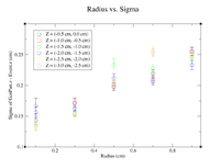
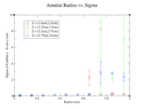
| + | Below is a plot and a table for the Radius vs. Sigma of GenPart.z - Event.z for several cuts in Z. For the plot each Radius is centered at the point plotted with a width of +/- 0.1 cm. | ||
| + | |||
| + | [[File:Radius vs sigma pos half.png|200px]] | ||
| + | |||
| + | {|border="5" | ||
| + | |- | ||
| + | || Z = (0.0 cm, 0.5 cm) | ||
| + | |- | ||
| + | ||R (cm) || 0.1 || 0.3 || 0.5 || 0.7 || 0.9 | ||
| + | |- | ||
| + | ||Sigma (cm) || 0.1548 +/- 0.0106 || 0.1825 +/- 0.0086 || 0.2167 +/- 0.0078 || 0.26 +/- 0.01 || 0.2774 +/- 0.0075 | ||
| + | |- | ||
| + | ||******************************************* | ||
| + | |- | ||
| + | || Z = (0.5 cm, 1.0 cm) | ||
| + | |- | ||
| + | ||R (cm) || 0.1 || 0.3 || 0.5 || 0.7 || 0.9 | ||
| + | |- | ||
| + | ||Sigma (cm) || 0.1672 +/- 0.0109 || 0.1636 +/- 0.0064 || 0.2277 +/- 0.0075 || 0.3203 +/- 0.0107 || 0.3287 +/- 0.0082 | ||
| + | |- | ||
| + | ||******************************************* | ||
| + | |- | ||
| + | ||Z = (1.0 cm, 1.5 cm) | ||
| + | |- | ||
| + | ||R (cm) || 0.1 || 0.3 || 0.5 || 0.7 || 0.9 | ||
| + | |- | ||
| + | ||Sigma (cm) || 0.1282 +/- 0.0068 || 0.1551 +/- 0.0042 || 0.1842 +/- 0.0052 || 0.2172 +/- 0.0069 || 0.2587 +/- 0.0072 | ||
| + | |- | ||
| + | ||******************************************* | ||
| + | |- | ||
| + | ||Z = (1.5 cm, 2.0 cm) | ||
| + | |- | ||
| + | ||R (cm) || 0.1 || 0.3 || 0.5 || 0.7 || 0.9 | ||
| + | |- | ||
| + | ||Sigma (cm) || 0.1264 +/- 0.0071 || 0.1558 +/- 0.0042 || 0.1795 +/- 0.0043 || 0.2034 +/- 0.0049 || 0.2391 +/- 0.0055 | ||
| + | |- | ||
| + | ||******************************************* | ||
| + | |- | ||
| + | ||Z = (2.0 cm, 2.5 cm) | ||
| + | |- | ||
| + | ||R (cm) || 0.1 || 0.3 || 0.5 || 0.7 || 0.9 | ||
| + | |- | ||
| + | ||Sigma (cm) || 0.1723 +/- 0.0120 || 0.1519 +/- 0.0038 || 0.1896 +/- 0.0048 || 0.2033 +/- 0.0043 || 0.2361 +/- 0.0048 | ||
| + | |- | ||
| + | ||******************************************* | ||
| + | |- | ||
| + | ||Z = (2.5 cm, 3.0 cm) | ||
| + | |- | ||
| + | ||R (cm) || 0.1 || 0.3 || 0.5 || 0.7 || 0.9 | ||
| + | |- | ||
| + | ||Sigma (cm) || 0.1273 +/- 0.0054 || 0.1665 +/- 0.0057 || 0.1936 +/- 0.0041 || 0.2143 +/- 0.0042 || 0.2337 +/- 0.0050 | ||
| + | |}<br> | ||
| + | |||
| + | Here is where the problem of a bimodal distribution become relevant as seen below in the histogram. | ||
| + | |||
| + | [[File:GenPart.z - Event.z bimodal example.png|200px]] | ||
| + | |||
| + | For now I will simply fit the larger peak to hopefully get rid of the muddling of the resolution, but this must be noted and investigated further later. | ||
| + | |||
| + | Below is the plot and the table for the negative half of the target. | ||
| + | |||
| + | [[File:Radius vs sigma neg half.png|200px]] | ||
| + | |||
| + | |||
| + | |||
| + | {|border="5" | ||
| + | |- | ||
| + | || Z = (-0.5 cm, 0.0 cm) | ||
| + | |- | ||
| + | ||R (cm) || 0.1 || 0.3 || 0.5 || 0.7 || 0.9 | ||
| + | |- | ||
| + | ||Sigma (cm) || 0.1666 +/- 0.0128 || 0.1722 +/- 0.0078 || 0.1983 +/- 0.0067 || 0.2193 +/- 0.0060 || 0.2554 +/- 0.0068 | ||
| + | |- | ||
| + | ||******************************************* | ||
| + | |- | ||
| + | || Z = (-1.0 cm, -0.5 cm) | ||
| + | |- | ||
| + | ||R (cm) || 0.1 || 0.3 || 0.5 || 0.7 || 0.9 | ||
| + | |- | ||
| + | ||Sigma (cm) || 0.1435 +/- 0.0069 || 0.1708 +/- 0.0068 || 0.2008 +/- 0.0069 || 0.2094 +/- 0.0058 || 0.2544 +/- 0.0065 | ||
| + | |- | ||
| + | ||******************************************* | ||
| + | |- | ||
| + | ||Z = (-1.5 cm, -1.0 cm) | ||
| + | |- | ||
| + | ||R (cm) || 0.1 || 0.3 || 0.5 || 0.7 || 0.9 | ||
| + | |- | ||
| + | ||Sigma (cm) || 0.1418 +/- 0.0073 || 0.1551 +/- 0.0047 || 0.2342 +/- 0.0092 || 0.2286 +/- 0.0066 || 0.2459 +/- 0.0066 | ||
| + | |- | ||
| + | ||******************************************* | ||
| + | |- | ||
| + | ||Z = (-2.0 cm, -1.5 cm) | ||
| + | |- | ||
| + | ||R (cm) || 0.1 || 0.3 || 0.5 || 0.7 || 0.9 | ||
| + | |- | ||
| + | ||Sigma (cm) || 0.1562 +/- 0.0091 || 0.1628 +/- 0.0045 || 0.2115 +/- 0.0076 || 0.2061 +/- 0.0056 || 0.2335 +/- 0.0077 | ||
| + | |- | ||
| + | ||******************************************* | ||
| + | |- | ||
| + | ||Z = (-2.5 cm, -2.0 cm) | ||
| + | |- | ||
| + | ||R (cm) || 0.1 || 0.3 || 0.5 || 0.7 || 0.9 | ||
| + | |- | ||
| + | ||Sigma (cm) || 0.1312 +/- 0.0059 || 0.1517 +/- 0.0040 || 0.2061 +/- 0.0049 || 0.257 +/- 0.008 || 0.2484 +/- 0.005 | ||
| + | |- | ||
| + | ||******************************************* | ||
| + | |- | ||
| + | ||Z = (-3.0 cm, -2.5 cm) | ||
| + | |- | ||
| + | ||R (cm) || 0.1 || 0.3 || 0.5 || 0.7 || 0.9 | ||
| + | |- | ||
| + | ||Sigma (cm) || 0.1339 +/- 0.0065 || 0.1539 +/- 0.0038 || 0.202 +/- 0.004 || 0.2537 +/- 0.0061 || 0.2517 +/- 0.0062 | ||
| + | |}<br> | ||
| + | |||
| + | It would seem that the bimodal distribution is having an effect on the results. It is counterintuitive that the resolution would get better the farther away from zero the events are. To begin investigating this, I made a Radius vs. Sigma plot for several values of Z. Here are some sample command lines in ROOT to get the width of the Gaussian peak. | ||
| + | |||
| + | |||
| + | clas12->Draw("Event.z >> (100,-5,5)","sqrt(GenPart.x*GenPart.x+GenPart.y*GenPart.y)<1.0 && sqrt(GenPart.x*GenPart.x+GenPart.y*GenPart.y)>0.8 && GenPart.z = 0"); | ||
| + | |||
| + | clas12->Draw("GenPart.z - Event.z >> (100,-5,5)","sqrt(GenPart.x*GenPart.x+GenPart.y*GenPart.y)<0.6 && sqrt(GenPart.x*GenPart.x+GenPart.y*GenPart.y)>0.4 && GenPart.z > 0.1 && GenPart.z < 0.5"); | ||
| + | |||
| + | clas12->Draw("GenPart.z - Event.z >> (100,-5,5)","sqrt(GenPart.x*GenPart.x+GenPart.y*GenPart.y)<0.6 && sqrt(GenPart.x*GenPart.x+GenPart.y*GenPart.y)>0.4 && GenPart.z > 0.5 && GenPart.z < 1.0"); | ||
| + | |||
| + | |||
| + | |||
| + | |||
| + | [[File:Radius vs Sigma Bimodal Investigation.png|200px]] | ||
| + | |||
| + | |||
| + | {|border="5" | ||
| + | |- | ||
| + | || Z = 0.0 cm | ||
| + | |- | ||
| + | ||R (cm) || 0.1 || 0.3 || 0.5 || 0.7 || 0.9 | ||
| + | |- | ||
| + | ||Sigma (cm) || 0.2873 +/- 0.0035 || 0.3457 +/- 0.0026 || 0.4045 +/- 0.0026 || 0.4466 +/- 0.0026 || 0.5359 +/- 0.0033 | ||
| + | |- | ||
| + | ||******************************************* | ||
| + | |- | ||
| + | || Z = (0.1 cm, 0.5 cm) | ||
| + | |- | ||
| + | ||R (cm) || 0.1 || 0.3 || 0.5 || 0.7 || 0.9 | ||
| + | |- | ||
| + | ||Sigma (cm) || 0.141 +/- 0.010 || 0.1651 +/- 0.0086 || 0.1991 +/- 0.0082 || 0.2572 +/- 0.0093 || 0.2676 +/- 0.0081 | ||
| + | |- | ||
| + | ||******************************************* | ||
| + | |- | ||
| + | ||Z = (0.5 cm, 1.0 cm) | ||
| + | |- | ||
| + | ||R (cm) || 0.1 || 0.3 || 0.5 || 0.7 || 0.9 | ||
| + | |- | ||
| + | ||Sigma (cm) || 0.1672 +/- 0.0109 || 0.1636 +/- 0.0064 || 0.2277 +/- 0.0075 || 0.3203 +/- 0.0107 || 0.3287 +/- 0.0082 | ||
| + | |- | ||
| + | |}<br> | ||
| + | |||
| + | |||
| + | To investigate the mystery as to why the resolution seems to get better as we move away from Z = 0 cm, I will plot create radius vs. sigma plots for different values of Z to try and pinpoint the problem. | ||
| + | |||
| + | Below is a link to the histograms for Z = 0 cm. A sample command line used is shown. | ||
| + | |||
| + | root [5] clas12->Draw("GenPart.z - Event.z >> (120,-6,6)","sqrt(GenPart.x*GenPart.x+GenPart.y*GenPart.y)<0.1 && sqrt(GenPart.x*GenPart.x+GenPart.y*GenPart.y)>0.0 && GenPart.z = 0"); | ||
| + | |||
| + | [[Histograms for Increasing Radii, Z = 0cm]] | ||
| + | |||
| + | [[File:Radius vs Sig GenPart.z=0.png|200px]] | ||
| + | |||
| + | Now that the Z = 0cm case has been done, the annular cuts will start to have a thickness of 0.25 cm in the Z direction. A sample command line in root is provided below. Notice that the annular thickness has been increased from 0.05 cm to 0.1 cm to increase the number of events in each histogram. | ||
| − | |||
| − | |||
| − | |||
| − | |||
| − | |||
| − | |||
| − | |||
| − | |||
| − | |||
| − | |||
| − | |||
| − | |||
| − | < | + | root [5] clas12->Draw("GenPart.z - Event.z >> (120,-6,6)","sqrt(GenPart.x*GenPart.x+GenPart.y*GenPart.y)<0.05 && sqrt(GenPart.x*GenPart.x+GenPart.y*GenPart.y)>0.0 && GenPart.z > 0 && GenPart.z < 0.25"); |
| − | + | [[Histograms for Increasing Radii, Z = (0.0cm,0.25cm)]] | |
| − | + | It would seem that the resolution when 0.6cm<R<0.7cm has failed completely. To double check on lds3 go to | |
| − | + | /home/lds/src/CLAS/GEMC/experiments/eg12/vertex/XYZRaster/Solenoid_On/30DegRot | |
| − | + | root -l eg12_sol_75k_2cm_XYRaster_6cm_ZRaster_30DegRot_rec_cat.root | |
| − | + | then use the command | |
| − | + | clas12->Draw("GenPart.z - Event.z>>(120,-6,6)","sqrt(GenPart.x*GenPart.x + GenPart.y*GenPart.y)>0.60 && sqrt(GenPart.x*GenPart.x + GenPart.y*GenPart.y)<0.70 && GenPart.z > 0.0 && GenPart.z<0.25"); | |
| + | Then by doing a Gaussian fit, the problem will appear. | ||
| − | + | [[Histograms for Increasing Radii, Z = (0.0cm,0.25cm)]] | |
| − | + | [[Histograms for Increasing Radii, Z = (0.25cm,0.5cm)]] | |
| − | |||
| − | |||
| − | |||
| − | |||
| − | |||
| − | |||
| − | |||
| − | |||
| − | + | [[Histograms for Increasing Radii, Z = (0.5cm,0.75cm)]] | |
| − | + | [[Histograms for Increasing Radii, Z = (0.75cm,1.0cm)]] | |
| − | + | [[Histograms for Increasing Radii, Z = (1.0cm,1.25cm)]] | |
| − | + | [[Histograms for Increasing Radii, Z = (1.25cm,1.5cm)]] | |
| − | [[ | + | [[Histograms for Increasing Radii, Z = (1.5cm,1.75cm)]] |
| − | + | [[Histograms for Increasing Radii, Z = (1.75cm,2.0cm)]] | |
| − | + | [[Histograms for Increasing Radii, Z = (2.0cm,2.25cm)]] | |
| − | + | [[Histograms for Increasing Radii, Z = (2.25cm,2.5cm)]] | |
| − | |||
| − | |||
| − | |||
| − | |||
| − | |||
| − | |||
| − | + | [[Histograms for Increasing Radii, Z = (2.5cm,2.75cm)]] | |
| + | [[Histograms for Increasing Radii, Z = (2.75cm,3.0cm)]] | ||
| − | + | In the histograms for increasing radii for Z = (-0.25cm,0.0cm) (not here yet), the histogram for 0.4cm<R<0.5cm seems very odd, but I verified it with root. Do a gaussian fit with the file eg12_sol_75k_2cm_XYRaster_6cm_ZRaster_30DegRot_rec_cat.root | |
| − | |||
| − | |||
| + | and use the command line | ||
| − | < | + | root [1] clas12->Draw("GenPart.z - Event.z>>(120,-6,6)","sqrt(GenPart.x*GenPart.x + GenPart.y*GenPart.y)>0.4 && sqrt(GenPart.x*GenPart.x + GenPart.y*GenPart.y)<0.5 && GenPart.z > -0.25 && GenPart.z<0.0"); |
| − | + | Below are the plots of the Annular Radius vs. Sigma for the negative half of the target. | |
| − | + | [[File:AnnularRad vs Sigma Z=(-1.0,0.0).png|200px]] | |
| + | [[File:AnnularRad vs Sigma Z=(-2.0,-1.0).png|200px]] | ||
| + | [[File:AnnularRad vs Sigma Z=-3.0,-2.0.png|200px]] | ||
| − | + | Here are the histograms for the positive half of the target | |
| − | + | [[File:AnnularRad vs sigma Z=0.0,1.0.png|200px]] | |
| + | [[File:Rad vs Sigma z=1.0,2.0.png|200px]] | ||
| + | [[File:Rad vs Sigma Z=2.0,3.0.png|200px]] | ||
| − | + | Now using GEMC 2.5 I will attempt to recreate the plots as seen in the JLAB wiki created by Dr. Forest. | |
| − | [[ | + | [[Recreation of Plots Using GEMC 2.5]] |
| + | [[Investigation of Centroid Shift in Vz Differences]] | ||
| − | + | =Elastic electron proton GEMC 2.4 & Coatjava 2.4= | |
=References= | =References= | ||
Latest revision as of 16:39, 11 November 2016
Vertex Reconstruction studies
Inclusive electron GEMC 2.4 & Coatjava 2.4
Summary
Set all histogram ranges to -6,6 cm and bin sizes of 0.1 cm
Below are some of the sample GEMC simulations as seen in the CED
There is a bash script on lds2 that will create Vx,Vy, and Vz differences for a point target, 3 2 cm line targets (in X,Y, and Z), 2 2D targets (one XZ target where X = 2cm and Z = 6cm and another where Y = 2cm and Z = 6 cm), and one 3D target where X = Y = 2cm and Z = 6cm. A 6 GeV electron is fired at angles degrees and degrees. The path to the script is /home/lds/src/CLAS/GEMC/experiments/eg12/vertex and the file is called run.exe. To run it you must be in a tcsh and have the setup in the GEMC directory sourced. Then simply hit ./run.exe. Right now the number of events is small (100), but that can easily be changed within the script.
Point target X,Y,Z=0 cm
The histograms below are using a 6 GeV electron fired at an angles of 25 degrees in theta and 0 degrees in phi.
For the plots below, I used the following gcard, sample LUND file, and commands in GEMC 2.4, coat-java 2.4, and ROOT
gcard:
<gcard>
      <detector name="../../../../clas12/fc/forwardCarriage" factory="TEXT" variation="original"/>
      <detector name="../../../../clas12/dc/dc"            factory="TEXT" variation="ccdb"/>
      <detector name="../../../../clas12/ec/ec"            factory="TEXT" variation="original"/>
      <detector name="../../../../clas12/ctof/ctof"            factory="TEXT" variation="original"/>
      <detector name="../../../../clas12/ftof/ftof"            factory="TEXT" variation="java"/>
      <detector name="../../../../clas12/htcc/htcc"            factory="TEXT" variation="original"/>
      <detector name="../../../../clas12/pcal/pcal"            factory="TEXT" variation="javageom"/>
      <detector name="../../../../clas12/magnets/solenoid" factory="TEXT" variation="original"/>
      <option name="SCALE_FIELD" value="clas12-torus-big, -1"/>
      <option name="HALL_FIELD"  value="clas12-solenoid"/>
      <option name="OUTPUT" value="evio,eg12_sol_75k_No_Raster.ev"/>
</gcard>
Sample LUND File:
1 1 1 1 1 1.00029 0.0718059 0.937771 1.48222 0.789865 1 -1 1 11 0 0 0 2.53564 5.43788 6 0.000511 0 0 0 1 1 1 1 1 1.00029 0.0718059 0.937771 1.48222 0.789865 1 -1 1 11 0 0 0 2.53564 5.43788 6 0.000511 0 0 0 1 1 1 1 1 1.00029 0.0718059 0.937771 1.48222 0.789865 1 -1 1 11 0 0 0 2.53564 5.43788 6 0.000511 0 0 0
GEMC Command:
~/src/CLAS/GEMC/source/gemc -USE_GUI=0 -INPUT_GEN_FILE="LUND,No_Raster.LUND" -N=75000 eg12_sol_No_Raster.gcard
Coat-Java 2.4 command:
~/src/CLAS/coatjava-2.4/bin/clas12-reconstruction -i ../files/vertex/vertex.evio -config GEOM::new=true -config MAG::torus=-1.0 -config MAG::solenoid=1.0 -o ../files/vertex/vertex_rec.evio -s DCHB:DCTB:EC:FTOF:EB -config DATA::mc=true -config DCTB::useRaster=true
Sample ROOT command:
clas12->Draw("GenPart.x - Event.x","abs(Event.x)<3");
| No Rastering | |
|---|---|
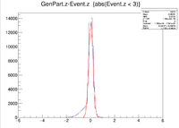
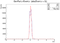
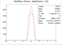
| Vx Difference | 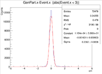
|
| Vy Difference | 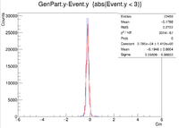
|
| Vz Difference | 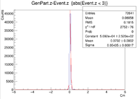
|
| X Resolution (cm) | 0.2362 +/- 0.0008 |
| Y Resolution(cm) | 0.09809 +/- 0.00033 |
| Z Resolution (cm) | 0.05435 +/- 0.00017 |
These histograms raise some questions. To begin I created a LUND file with 6 GeV incident electrons at 25 degrees in theta and 0 degrees in phi. All of the vertex positions were set to 0. I then ran GEMC 2.4 using the command line ~/src/CLAS/GEMC/source/gemc -USE_GUI=0 -INPUT_GEN_FILE="LUND,No_Raster.LUND" -N=75000 eg12_sol_No_Raster.gcard
which created an output file called eg12_sol_75k_No_Raster.ev. After that the reconstruction command line used was
~/src/CLAS/coatjava-2.4/bin/clas12-reconstruction -i eg12_sol_75k_No_Raster.ev-config GEOM::new=true -config MAG::torus=-1.0 -config MAG::solenoid=1.0 -o eg12_sol_75k_No_Raster_rec.evio -s DCHB:DCTB:EC:FTOF:EB -config DATA::mc=true -config DCTB::useRaster=true
After the reconstruction a root file was created using
~/src/CLAS/evio2root/bin/evio2root eg12_sol_75k_No_Raster_rec.evio eg12_sol_75k_No_Raster_rec.root 75000
A plot was then created to show the X Vertex and Y Vertex Differences
The first question is why is there a shift in the Y Difference. What would make X more centered around 0? The next question is when rastering begins, why do the resolutions in the X Vertices remain unchanged while the resolutions in the Y Vertices change?
Point in 2-D but extended target in 1-D
Two vertex variables are fixed at zero and the third vertex variable is altered. A 6 GeV electron was fired at angles of 25 degrees in theta and 0 degrees in phi.
The gcard used had the same detector parts as above, but the filename and pathways were changed.
Below is a sample line from the LUND files:
For 2cm X Target: 1 1 1 1 1 1.00029 0.0718059 0.937771 1.48222 0.789865 1 -1 1 11 0 0 0 2.53564 5.43788 6 0.000511 0.999484 0 0
For 2cm Y Target: 1 1 1 1 1 1.00029 0.0718059 0.937771 1.48222 0.789865 1 -1 1 11 0 0 0 2.53564 5.43788 6 0.000511 0 0.999484 0
For 2cm Z Target: 1 1 1 1 1 1.00029 0.0718059 0.937771 1.48222 0.789865 1 -1 1 11 0 0 0 2.53564 5.43788 6 0.000511 0 0 2.99845
Also, here are the GEMC, Coat-Java, and a sample ROOT command.
GEMC: ~/src/CLAS/GEMC/source/gemc -USE_GUI=0 -INPUT_GEN_FILE="LUND,test.LUND" -N=100 eg12.gcard
Coat-Java:~/src/CLAS/coatjava-2.4/bin/clas12-reconstruction -i ../files/vertex/vertex.evio -config GEOM::new=true -config MAG::torus=-1.0 -config MAG::solenoid=1.0 -o ../files/vertex/vertex_rec.evio -s DCHB:DCTB:EC:FTOF:EB -config DATA::mc=true -config DCTB::useRaster=true
Sample ROOT command: clas12->Draw("GenPart.x - Event.x","abs(Event.x)<2");
Extended target -3 < Z < 3 cm
For the plots below a 6 GeV electron was fired at angles theta = 25 degrees and phi = 0 degrees. There were 3 separate simulations ran for when -3 cm < Z < 3 cm. The first was a 2-D target with -3 cm < Z < 3 cm and -1 cm < X < 1 cm and Y = 0 cm, while the second had the same values for Z, but instead -1 cm < Y < 1cm and X = 0 cm. The final set of plots was created using -3 cm < Z < 3 cm , -1 cm < X < 1 cm, and -1 cm < Y < 1 cm.
Below are some of the sample LUND files used.
For the XZ Target:
1 1 1 1 1 1.00029 0.0718059 0.937771 1.48222 0.789865 1 -1 1 11 0 0 0 2.53564 5.43788 6 0.000511 -0.67418 0 2.99845 1 1 1 1 1 1.00029 0.0718059 0.937771 1.48222 0.789865 1 -1 1 11 0 0 0 2.53564 5.43788 6 0.000511 0.894402 0 -1.30429
For the YZ Target:
1 1 1 1 1 1.00029 0.0718059 0.937771 1.48222 0.789865 1 -1 1 11 0 0 0 2.53564 5.43788 6 0.000511 0 -0.67418 2.99845 1 1 1 1 1 1.00029 0.0718059 0.937771 1.48222 0.789865 1 -1 1 11 0 0 0 2.53564 5.43788 6 0.000511 0 0.894402 -1.30429
For the XYZ Target:
1 1 1 1 1 1.00029 0.0718059 0.937771 1.48222 0.789865 1 -1 1 11 0 0 0 2.53564 5.43788 6 0.000511 -0.67418 -0.434764 2.99845 1 1 1 1 1 1.00029 0.0718059 0.937771 1.48222 0.789865 1 -1 1 11 0 0 0 2.53564 5.43788 6 0.000511 -0.536687 -0.0300528 2.68321 1 1 1 1 1 1.00029 0.0718059 0.937771 1.48222 0.789865 1 -1 1 11 0 0 0 2.53564 5.43788 6 0.000511 0.488611 0.0800873 2.74486
The GEMC and Coat-Java command lines are similar to the previously seen commands. The only things that changed were the LUND file names, and the ev/evio filenames. The command lines can be seen at the top of the histograms.
VertREC_9-22-16_table_3ltZgt-3
Extended target in Z. Vy shift analysis
All Histograms below were created by simply making the target longer along the Z axis. Each case uses vertex points for X and Y ranging from -1cm to 1cm
VertREC_9-22-16_table_3ltZgt-3_1gtRlt-1
Localized Vertex Resolution Investigation of Line Targets
GEMC was ran to create electrons being produced in a line along certain axes. These include three separate 2cm targets centered at (0,0,0) in the X, Y , and Z directions. The final target is a line along the Z axis centered at (0,0,0) that is 6cm long. The generated electrons were shot at 25 degrees in theta and 0 degrees in phi at an energy of 6GeV.
Here is an example of how the cuts were made. Consider the case of a 2cm line target in the Z direction centered at (0,0,0). Closed intervals begin at the end of the target and are 0.1cm long. So the first interval would be [-1.0,-0.9], then the next would be [-0.9, -0.8] and so on until the entire target is covered. The events in the EVENTHB bank were cut so that in any given interval there would be a margin of +/- 1cm from the end of the area of interest to remove any outliers that may cause the histograms to have long tails.
Below are the histograms for the 2cm line target in Y,X=0,Z=0. The electrons were fired with an energy of 6 GeV at 25 degrees in theta at 0 degrees in phi.
2cm YLineTarg 0 Degree Rotation 09/23/16
Below are the histograms for a 2cm target along the Y axis, X = 0 Z = 0. The electrons were fired with an energy of 6 GeV at 25 degrees in theta and 180 degrees in phi.
2cm YLineTarg 180 Degree Rotation 09/23/16
Below are the Histograms for a 2cm long target in the X Direction with a 6GeV electron fired at 25 degrees in theta and 90 degrees in phi
2cm XLineTarg 90 Degree Rotation 09/23/16
Below are the Vx Differences using a 2cm target in X with incident 6 GeV electrons at 25 degrees in theta and 270 degrees in phi
2cm XLineTarg 270 Degree Rotation 09/23/16
Below are the histograms for a 6cm target in the Z direction using a 6 GeV electron fired at 25 degrees in theta and 0 degrees in phi.
6cm ZLineTarg 0 Degree Rotation 09/23/16
Below are the histograms for a 6cm target in the Z direction using a 6 GeV electron fired at 25 degrees in theta and 90 degrees in phi.
6cm ZLineTarg 90 Degree Rotation 09/23/16
Below are the histograms for a 6 GeV electron fired at angles 25 degrees in theta and 270 degrees in phi. The target was 6cm in the Z direction.
6cm ZLineTarg 270 Degree Rotation 09/23/16
Below are the histograms for a 2cm target along the Y axis, X = 0 Z = 0. The electrons were fired with an energy of 6 GeV at 25 degrees in theta and 30 degrees in phi.
2cm YLineTarg 30 Degree Rotation 09/23/16
Below are the histograms for a 2cm Y target with an incident electron energy of 6 GeV. The angles were theta = 25 degrees and phi = 210 degrees
2cm YLineTarg 210 Degree Rotation 09/23/16
Localized Vertex Resolution Investigation of 2 Dimensional Targets
The histograms below were created using a 6 GeV electron fired at 25 degrees in theta and 30 degrees in phi. To make the cuts I simply made circles of increasing radius centered at the origin. I used 0.1cm increments to make the 10 histograms for each vertex position.
Below are the Vx and Vy Differences for a 2cm XY target, Z=0.
2cm XYTarg Z=0 Vx and Vy Differences 09/23/16
Below are the Vy and Vz differences for a 2cm target in Y and Z, X=0. The electrons were fired with an energy of 6 GeV and angles of 25 degrees in theta and 30 degrees in phi.
2cm YZTarg X=0 Vz and Vy Difference 09/23/16
Below are the Vx and Vz differences for a 2cm XZ target, Y = 0. The electrons were fired with an energy of 6 GeV at angles theta = 25 degrees and phi = 30 degrees.
2cm XZTarg Y=0 Vx and Vz Differences 09/23/16
Localized Vertex Resolution of 3 Dimensional targets
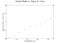
For the plots below, a 6 GeV electron was fired at angles 25 degrees in theta and 30 degrees in phi. The target has an XY radius of 1cm and a length in the Z direction of 6cm. Setting GenPart.z = 0cm, the resolution was investigated as a function of the target's XY radius along with a table for the values.
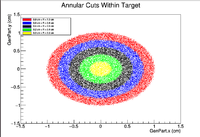
In this section, concentric rings with a thickness of 0.1cm were created within the target. For example these plots would include a ring centered at x=y=z=0 and include all GenPart.x and GenPart.y from (0.0 cm, 0.1 cm), then another ring would include all Genpart.x and GenPart.y events from (0.1 cm, 0.2 cm) and so on until we reach the edge of the target. Below is a visualization of the cuts as seen in a 2D cross section of the target.
clas12->Draw("Event.z >> (100,-5,5)","sqrt(GenPart.x*GenPart.x+GenPart.y*GenPart.y)<0.95 && sqrt(GenPart.x*GenPart.x+GenPart.y*GenPart.y)>0.85");
| R (cm) | 0.05 +/- 0.05 | 0.15 +/- 0.05 | 0.25 +/- 0.05 | 0.35 +/- 0.05 | 0.45 +/- 0.05 | 0.55 +/- 0.05 | 0.65 +/- 0.05 | 0.75 +/- 0.05 | 0.85 +/- 0.05 | 0.95 +/- 0.05 |
| Width (cm) | 0.05094 +/- 0.0019 | 0.07812 +/- 0.0018 | 0.3688 +/- 0.0063 | 0.5231 +/- 0.0077 | 0.718 +/- 0.012 | 0.7987 +/- 0.0092 | 0.8709 +/- 0.0085 | 1.038 +/- 0.01 | 1.183 +/- 0.012 | 1.296 +/- 0.013 |
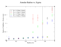
For the next set of plots, the GEMC simulations had the same energy and angles as above. To construct scatter plots, similar annular cuts in the radius were made (similar to above), but this time the thickness of each ring was 0.2 cm (to ensure enough events were present). In addition, the target will become extended in Z. Cuts were made in Z by restricting GenPart.z to be within a range of certain values. Each "washer" shape has a thickness of 0.5 cm in the Z direction. Histograms were created using the following command line as an example
clas12->Draw("GenPart.z - Event.z >> (100,-5,5)","sqrt(GenPart.x*GenPart.x+GenPart.y*GenPart.y)<0.2 && sqrt(GenPart.x*GenPart.x+GenPart.y*GenPart.y)>0.0 && GenPart.z > 0.0 && GenPart.z < 0.5");
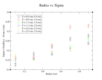
Below is a plot and a table for the Radius vs. Sigma of GenPart.z - Event.z for several cuts in Z. For the plot each Radius is centered at the point plotted with a width of +/- 0.1 cm.
| Z = (0.0 cm, 0.5 cm) | |||||
| R (cm) | 0.1 | 0.3 | 0.5 | 0.7 | 0.9 |
| Sigma (cm) | 0.1548 +/- 0.0106 | 0.1825 +/- 0.0086 | 0.2167 +/- 0.0078 | 0.26 +/- 0.01 | 0.2774 +/- 0.0075 |
| ******************************************* | |||||
| Z = (0.5 cm, 1.0 cm) | |||||
| R (cm) | 0.1 | 0.3 | 0.5 | 0.7 | 0.9 |
| Sigma (cm) | 0.1672 +/- 0.0109 | 0.1636 +/- 0.0064 | 0.2277 +/- 0.0075 | 0.3203 +/- 0.0107 | 0.3287 +/- 0.0082 |
| ******************************************* | |||||
| Z = (1.0 cm, 1.5 cm) | |||||
| R (cm) | 0.1 | 0.3 | 0.5 | 0.7 | 0.9 |
| Sigma (cm) | 0.1282 +/- 0.0068 | 0.1551 +/- 0.0042 | 0.1842 +/- 0.0052 | 0.2172 +/- 0.0069 | 0.2587 +/- 0.0072 |
| ******************************************* | |||||
| Z = (1.5 cm, 2.0 cm) | |||||
| R (cm) | 0.1 | 0.3 | 0.5 | 0.7 | 0.9 |
| Sigma (cm) | 0.1264 +/- 0.0071 | 0.1558 +/- 0.0042 | 0.1795 +/- 0.0043 | 0.2034 +/- 0.0049 | 0.2391 +/- 0.0055 |
| ******************************************* | |||||
| Z = (2.0 cm, 2.5 cm) | |||||
| R (cm) | 0.1 | 0.3 | 0.5 | 0.7 | 0.9 |
| Sigma (cm) | 0.1723 +/- 0.0120 | 0.1519 +/- 0.0038 | 0.1896 +/- 0.0048 | 0.2033 +/- 0.0043 | 0.2361 +/- 0.0048 |
| ******************************************* | |||||
| Z = (2.5 cm, 3.0 cm) | |||||
| R (cm) | 0.1 | 0.3 | 0.5 | 0.7 | 0.9 |
| Sigma (cm) | 0.1273 +/- 0.0054 | 0.1665 +/- 0.0057 | 0.1936 +/- 0.0041 | 0.2143 +/- 0.0042 | 0.2337 +/- 0.0050 |
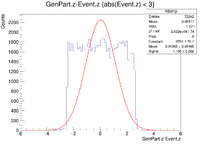
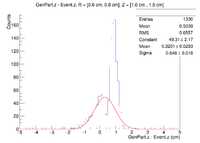
Here is where the problem of a bimodal distribution become relevant as seen below in the histogram.
For now I will simply fit the larger peak to hopefully get rid of the muddling of the resolution, but this must be noted and investigated further later.
Below is the plot and the table for the negative half of the target.
| Z = (-0.5 cm, 0.0 cm) | |||||
| R (cm) | 0.1 | 0.3 | 0.5 | 0.7 | 0.9 |
| Sigma (cm) | 0.1666 +/- 0.0128 | 0.1722 +/- 0.0078 | 0.1983 +/- 0.0067 | 0.2193 +/- 0.0060 | 0.2554 +/- 0.0068 |
| ******************************************* | |||||
| Z = (-1.0 cm, -0.5 cm) | |||||
| R (cm) | 0.1 | 0.3 | 0.5 | 0.7 | 0.9 |
| Sigma (cm) | 0.1435 +/- 0.0069 | 0.1708 +/- 0.0068 | 0.2008 +/- 0.0069 | 0.2094 +/- 0.0058 | 0.2544 +/- 0.0065 |
| ******************************************* | |||||
| Z = (-1.5 cm, -1.0 cm) | |||||
| R (cm) | 0.1 | 0.3 | 0.5 | 0.7 | 0.9 |
| Sigma (cm) | 0.1418 +/- 0.0073 | 0.1551 +/- 0.0047 | 0.2342 +/- 0.0092 | 0.2286 +/- 0.0066 | 0.2459 +/- 0.0066 |
| ******************************************* | |||||
| Z = (-2.0 cm, -1.5 cm) | |||||
| R (cm) | 0.1 | 0.3 | 0.5 | 0.7 | 0.9 |
| Sigma (cm) | 0.1562 +/- 0.0091 | 0.1628 +/- 0.0045 | 0.2115 +/- 0.0076 | 0.2061 +/- 0.0056 | 0.2335 +/- 0.0077 |
| ******************************************* | |||||
| Z = (-2.5 cm, -2.0 cm) | |||||
| R (cm) | 0.1 | 0.3 | 0.5 | 0.7 | 0.9 |
| Sigma (cm) | 0.1312 +/- 0.0059 | 0.1517 +/- 0.0040 | 0.2061 +/- 0.0049 | 0.257 +/- 0.008 | 0.2484 +/- 0.005 |
| ******************************************* | |||||
| Z = (-3.0 cm, -2.5 cm) | |||||
| R (cm) | 0.1 | 0.3 | 0.5 | 0.7 | 0.9 |
| Sigma (cm) | 0.1339 +/- 0.0065 | 0.1539 +/- 0.0038 | 0.202 +/- 0.004 | 0.2537 +/- 0.0061 | 0.2517 +/- 0.0062 |
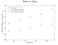
It would seem that the bimodal distribution is having an effect on the results. It is counterintuitive that the resolution would get better the farther away from zero the events are. To begin investigating this, I made a Radius vs. Sigma plot for several values of Z. Here are some sample command lines in ROOT to get the width of the Gaussian peak.
clas12->Draw("Event.z >> (100,-5,5)","sqrt(GenPart.x*GenPart.x+GenPart.y*GenPart.y)<1.0 && sqrt(GenPart.x*GenPart.x+GenPart.y*GenPart.y)>0.8 && GenPart.z = 0");
clas12->Draw("GenPart.z - Event.z >> (100,-5,5)","sqrt(GenPart.x*GenPart.x+GenPart.y*GenPart.y)<0.6 && sqrt(GenPart.x*GenPart.x+GenPart.y*GenPart.y)>0.4 && GenPart.z > 0.1 && GenPart.z < 0.5");
clas12->Draw("GenPart.z - Event.z >> (100,-5,5)","sqrt(GenPart.x*GenPart.x+GenPart.y*GenPart.y)<0.6 && sqrt(GenPart.x*GenPart.x+GenPart.y*GenPart.y)>0.4 && GenPart.z > 0.5 && GenPart.z < 1.0");
| Z = 0.0 cm | |||||
| R (cm) | 0.1 | 0.3 | 0.5 | 0.7 | 0.9 |
| Sigma (cm) | 0.2873 +/- 0.0035 | 0.3457 +/- 0.0026 | 0.4045 +/- 0.0026 | 0.4466 +/- 0.0026 | 0.5359 +/- 0.0033 |
| ******************************************* | |||||
| Z = (0.1 cm, 0.5 cm) | |||||
| R (cm) | 0.1 | 0.3 | 0.5 | 0.7 | 0.9 |
| Sigma (cm) | 0.141 +/- 0.010 | 0.1651 +/- 0.0086 | 0.1991 +/- 0.0082 | 0.2572 +/- 0.0093 | 0.2676 +/- 0.0081 |
| ******************************************* | |||||
| Z = (0.5 cm, 1.0 cm) | |||||
| R (cm) | 0.1 | 0.3 | 0.5 | 0.7 | 0.9 |
| Sigma (cm) | 0.1672 +/- 0.0109 | 0.1636 +/- 0.0064 | 0.2277 +/- 0.0075 | 0.3203 +/- 0.0107 | 0.3287 +/- 0.0082 |
To investigate the mystery as to why the resolution seems to get better as we move away from Z = 0 cm, I will plot create radius vs. sigma plots for different values of Z to try and pinpoint the problem.
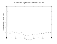
Below is a link to the histograms for Z = 0 cm. A sample command line used is shown.
root [5] clas12->Draw("GenPart.z - Event.z >> (120,-6,6)","sqrt(GenPart.x*GenPart.x+GenPart.y*GenPart.y)<0.1 && sqrt(GenPart.x*GenPart.x+GenPart.y*GenPart.y)>0.0 && GenPart.z = 0");
Histograms for Increasing Radii, Z = 0cm
Now that the Z = 0cm case has been done, the annular cuts will start to have a thickness of 0.25 cm in the Z direction. A sample command line in root is provided below. Notice that the annular thickness has been increased from 0.05 cm to 0.1 cm to increase the number of events in each histogram.
root [5] clas12->Draw("GenPart.z - Event.z >> (120,-6,6)","sqrt(GenPart.x*GenPart.x+GenPart.y*GenPart.y)<0.05 && sqrt(GenPart.x*GenPart.x+GenPart.y*GenPart.y)>0.0 && GenPart.z > 0 && GenPart.z < 0.25");
Histograms for Increasing Radii, Z = (0.0cm,0.25cm)
It would seem that the resolution when 0.6cm<R<0.7cm has failed completely. To double check on lds3 go to
/home/lds/src/CLAS/GEMC/experiments/eg12/vertex/XYZRaster/Solenoid_On/30DegRot
root -l eg12_sol_75k_2cm_XYRaster_6cm_ZRaster_30DegRot_rec_cat.root
then use the command
clas12->Draw("GenPart.z - Event.z>>(120,-6,6)","sqrt(GenPart.x*GenPart.x + GenPart.y*GenPart.y)>0.60 && sqrt(GenPart.x*GenPart.x + GenPart.y*GenPart.y)<0.70 && GenPart.z > 0.0 && GenPart.z<0.25");
Then by doing a Gaussian fit, the problem will appear.
Histograms for Increasing Radii, Z = (0.0cm,0.25cm)
Histograms for Increasing Radii, Z = (0.25cm,0.5cm)
Histograms for Increasing Radii, Z = (0.5cm,0.75cm)
Histograms for Increasing Radii, Z = (0.75cm,1.0cm)
Histograms for Increasing Radii, Z = (1.0cm,1.25cm)
Histograms for Increasing Radii, Z = (1.25cm,1.5cm)
Histograms for Increasing Radii, Z = (1.5cm,1.75cm)
Histograms for Increasing Radii, Z = (1.75cm,2.0cm)
Histograms for Increasing Radii, Z = (2.0cm,2.25cm)
Histograms for Increasing Radii, Z = (2.25cm,2.5cm)
Histograms for Increasing Radii, Z = (2.5cm,2.75cm)
Histograms for Increasing Radii, Z = (2.75cm,3.0cm)
In the histograms for increasing radii for Z = (-0.25cm,0.0cm) (not here yet), the histogram for 0.4cm<R<0.5cm seems very odd, but I verified it with root. Do a gaussian fit with the file eg12_sol_75k_2cm_XYRaster_6cm_ZRaster_30DegRot_rec_cat.root
and use the command line
root [1] clas12->Draw("GenPart.z - Event.z>>(120,-6,6)","sqrt(GenPart.x*GenPart.x + GenPart.y*GenPart.y)>0.4 && sqrt(GenPart.x*GenPart.x + GenPart.y*GenPart.y)<0.5 && GenPart.z > -0.25 && GenPart.z<0.0");
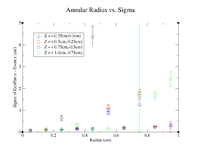
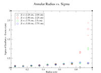
Below are the plots of the Annular Radius vs. Sigma for the negative half of the target.
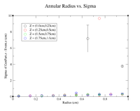
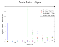
Here are the histograms for the positive half of the target
Now using GEMC 2.5 I will attempt to recreate the plots as seen in the JLAB wiki created by Dr. Forest.
Recreation of Plots Using GEMC 2.5
Investigation of Centroid Shift in Vz Differences
Elastic electron proton GEMC 2.4 & Coatjava 2.4
References
https://clasweb.jlab.org/wiki/index.php/TF_EG12_Vertex#Z_resolution_With_micro-megas
