Difference between revisions of "Relative efficiency"
| (161 intermediate revisions by the same user not shown) | |||
| Line 1: | Line 1: | ||
| − | + | Some papers | |
| + | |||
| + | [[File:nn_correlation_extraction.pdf]] | ||
| + | |||
| + | |||
| + | [[File:Ynn_vs_Dnn.pdf]] | ||
| + | |||
| + | |||
| + | |||
| + | ==Rletive efficiency obtained from the 2n opening angle w/ uncorrelated neutrons== | ||
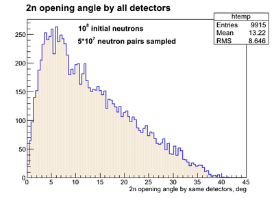
The result of simulation of 2n openeing angle obtained by different neutron detectors (each neutron hit different detector) having y-resolution is presented below. The source of neutrons was isotropic. | The result of simulation of 2n openeing angle obtained by different neutron detectors (each neutron hit different detector) having y-resolution is presented below. The source of neutrons was isotropic. | ||
| − | [[File:2n_op_angle_all_diffDets.png || 400px]] | + | |
| + | |||
| + | |||
| + | {| cellpadding="2" style="border: 1px solid darkgray;" | ||
| + | ! width="400" | Empty target, <math>10^8</math> events sampled | ||
| + | ! width="400" | DU target, <math>10^8</math> events sampled | ||
| + | |- border="0" | ||
| + | | [[File:2n_op_angle_all_diffDets.png|400px|Region 1]] | ||
| + | | [[File:2n_op_angle_all_diffDets_DUmat.png|400px|Region 2]] | ||
| + | |- align="center" | ||
| + | | Point isotropic n-source w/o material || Volume isotropic n-source + DU material | ||
| + | |} | ||
The result of simulation of 2n openeing angle obtained by the same neutron detectors (2 neutrons hit same detector) having y-resolution is presented below: | The result of simulation of 2n openeing angle obtained by the same neutron detectors (2 neutrons hit same detector) having y-resolution is presented below: | ||
| Line 12: | Line 32: | ||
[[File:relative_effcy_diff_pulses.png || 800px]] | [[File:relative_effcy_diff_pulses.png || 800px]] | ||
| + | |||
| + | ==Relative efficiency of the detecting system obtained using experimental data only (all runs)== | ||
| + | |||
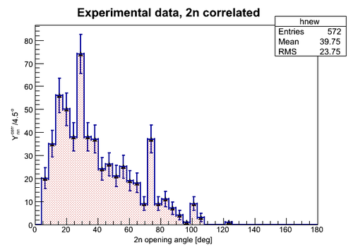
| + | In this part the experimantal data are presented for the cases when (1) the 2n opening angle was measured for neutrons correlated and (2) the 2n opening angle was measured for neutrons uncorrelated (neutrons from separate pulses). In the figure below the experimental data on the 2n opening angle measured for the case of correlated neutrons is presented where the statistical error bar width is equal to <math>\pm \sqrt{N_{bin}}</math> along y-axis and 4.5 deg along x-axis (the bin width). The total number of triggering pulses during the experiment was Nexp_pulses=2.469256E+7. | ||
| + | |||
| + | [[File:exp_data_2n_correlated_Err.png || 500px]] | ||
| + | |||
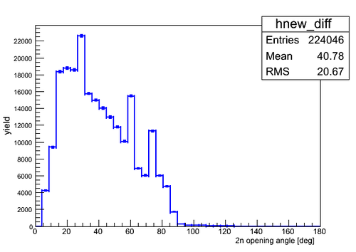
| + | The experimental data on the 2n opening angle measured for the case of uncorrelated neutrons is presented in the next figure. 80 neutrons from different pulses were taken uniformly to reproduce 2n opening angle for the case of uncorrelated neutrons. The total number of uncorrelated neutron pairs was Npair_uncorr = 3.608397E+7. The width of the error bars is smaller then the size of the markers. | ||
| + | |||
| + | [[File:exp_data_2n_uncorrelated_Err2.png || 500px]] | ||
| + | |||
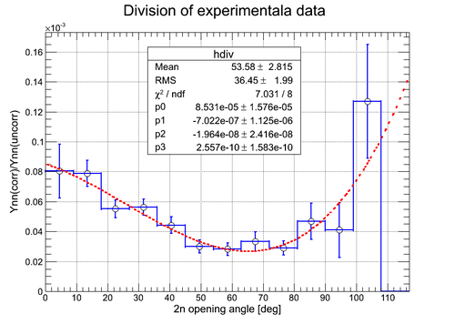
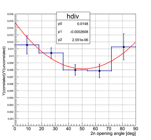
| + | The result of the division of the two histograms (<math>Y_{nn}^{correlated}/Y_{nn}^{uncorrelated}</math>) obtained for the described two cases is shown below. In order to obtain the resulting histogram as a division of the previous two histograms we need to do the division on the bin-by-bin basis as <math>\frac{a \pm \delta a}{b \pm \delta b}</math>, where <math>a</math> and <math>b</math> are the contents of the corresponding bins and <math>\delta a</math> and <math>\delta b</math> are the coresponding statistical errors for the bin contents <math>a</math> and <math>b</math>. The error bars were obtained by the propagation in the following way: <math>\delta Err = \frac{a}{b}\sqrt{(\frac{\delta a}{a})^2+(\frac{\delta b}{b})^2}</math>. The resulting histogram wa normalized to the ratio of the total number of pulses to the total number of uncorrelated neutron pairs considered Norm = Nexp_pulses/Npair_uncorr = 2.469256E+7/3.608397E+7 . It should be noted that the total number of uncorrelated neutron pairs can be varied by changing the number of corresponding combinations and the number of pulses involved into the 2n opening angle reproduction, so the normalization may change. | ||
| + | |||
| + | [[File:corr_over_uncorr_fit.png || 500px]] | ||
| + | |||
| + | ==Normalization== | ||
| + | |||
| + | Data table 1. | ||
| + | |||
| + | {| class="wikitable" | ||
| + | ! style="text-align: center;" | run# | ||
| + | ! style="text-align: center;" | Total # of pulses per run | ||
| + | |- | ||
| + | | style="text-align: center;" | run4118 | ||
| + | | style="text-align: center;" | 1668482 | ||
| + | |- | ||
| + | | style="text-align: center;" | run4119 | ||
| + | | style="text-align: center;" | 2135901 | ||
| + | |- | ||
| + | | style="text-align: center;" | run4133 | ||
| + | | style="text-align: center;" | 1704331 | ||
| + | |- | ||
| + | | style="text-align: center;" | run4134 | ||
| + | | style="text-align: center;" | 1732490 | ||
| + | |- | ||
| + | | style="text-align: center;" | run4135 | ||
| + | | style="text-align: center;" | 1603604 | ||
| + | |- | ||
| + | | style="text-align: center;" | run4137 | ||
| + | | style="text-align: center;" | 800699 | ||
| + | |- | ||
| + | | style="text-align: center;" | run4144 | ||
| + | | style="text-align: center;" | 1645667 | ||
| + | |- | ||
| + | | style="text-align: center;" | run4145 | ||
| + | | style="text-align: center;" | 1544605 | ||
| + | |- | ||
| + | | style="text-align: center;" | run4146 | ||
| + | | style="text-align: center;" | 510826 | ||
| + | |- | ||
| + | | style="text-align: center;" | run4153 | ||
| + | | style="text-align: center;" | 1750657 | ||
| + | |- | ||
| + | | style="text-align: center;" | run4154 | ||
| + | | style="text-align: center;" | 1631436 | ||
| + | |- | ||
| + | | style="text-align: center;" | run4155 | ||
| + | | style="text-align: center;" | 1062048 | ||
| + | |- | ||
| + | | style="text-align: center;" | run4166 | ||
| + | | style="text-align: center;" | 214600 | ||
| + | |- | ||
| + | | style="text-align: center;" | run4169 | ||
| + | | style="text-align: center;" | 191592 | ||
| + | |- | ||
| + | | style="text-align: center;" | run4170 | ||
| + | | style="text-align: center;" | 429974 | ||
| + | |- | ||
| + | | style="text-align: center;" | run4171 | ||
| + | | style="text-align: center;" | 1141113 | ||
| + | |- | ||
| + | | style="text-align: center;" | run4172 | ||
| + | | style="text-align: center;" | 650734 | ||
| + | |- | ||
| + | | style="text-align: center;" | run4173 | ||
| + | | style="text-align: center;" | 354992 | ||
| + | |- | ||
| + | | style="text-align: center;" | run4174 | ||
| + | | style="text-align: center;" | 953831 | ||
| + | |- | ||
| + | | style="text-align: center;" | run4175 | ||
| + | | style="text-align: center;" | 299086 | ||
| + | |- | ||
| + | | style="text-align: center;" | run4176 | ||
| + | | style="text-align: center;" | 144774 | ||
| + | |- | ||
| + | | style="text-align: center;" | run4177 | ||
| + | | style="text-align: center;" | 225877 | ||
| + | |- | ||
| + | | style="text-align: center;" | run4203 | ||
| + | | style="text-align: center;" | 659050 | ||
| + | |- | ||
| + | | style="text-align: center;" | run4204 | ||
| + | | style="text-align: center;" | 1636192 | ||
| + | |- | ||
| + | | style="text-align: center;" | totals | ||
| + | | style="text-align: center; background: red; color: white" | 24692561 | ||
| + | |} | ||
| + | |||
| + | Normalization factor is 24692561. | ||
| + | |||
| + | [[File:2n_corr_opAngle_normalized.png | 500px]] | ||
| + | |||
| + | Data table 2. Uncorrelated neutron pairs. | ||
| + | |||
| + | {| class="wikitable" | ||
| + | ! style="text-align: center;" | run# | ||
| + | ! style="text-align: center;" | 80 puls pairs | ||
| + | ! style="text-align: center;" | all nonZ pairs | ||
| + | ! style="text-align: center;" | total # of pairs | ||
| + | |- | ||
| + | | style="text-align: center;" | run4118 | ||
| + | | style="text-align: center;" | 1949796 | ||
| + | | style="text-align: center;" | 35168980 | ||
| + | | style="text-align: center;" | 58460510939894 | ||
| + | |- | ||
| + | | style="text-align: center;" | run4119 | ||
| + | | style="text-align: center;" | 2470399 | ||
| + | | style="text-align: center;" | 57115623 | ||
| + | | style="text-align: center;" | 95803579611944 | ||
| + | |- | ||
| + | | style="text-align: center;" | run4133 | ||
| + | | style="text-align: center;" | 1741760 | ||
| + | | style="text-align: center;" | 30145143 | ||
| + | | style="text-align: center;" | 60999663129029 | ||
| + | |- | ||
| + | | style="text-align: center;" | run4134 | ||
| + | | style="text-align: center;" | 1832885 | ||
| + | | style="text-align: center;" | 33384324 | ||
| + | | style="text-align: center;" | 63031990015343 | ||
| + | |- | ||
| + | | style="text-align: center;" | run4135 | ||
| + | | style="text-align: center;" | 1727993 | ||
| + | | style="text-align: center;" | 28580648 | ||
| + | | style="text-align: center;" | 54002495269034 | ||
| + | |- | ||
| + | | style="text-align: center;" | run4137 | ||
| + | | style="text-align: center;" | 833189 | ||
| + | | style="text-align: center;" | 7099684 | ||
| + | | style="text-align: center;" | 13463513489481 | ||
| + | |- | ||
| + | | style="text-align: center;" | run4144 | ||
| + | | style="text-align: center;" | 1770693 | ||
| + | | style="text-align: center;" | 26603021 | ||
| + | | style="text-align: center;" | 56872651957830 | ||
| + | |- | ||
| + | | style="text-align: center;" | run4145 | ||
| + | | style="text-align: center;" | 1592222 | ||
| + | | style="text-align: center;" | 20562899 | ||
| + | | style="text-align: center;" | 50101929186175 | ||
| + | |- | ||
| + | | style="text-align: center;" | run4146 | ||
| + | | style="text-align: center;" | 491705 | ||
| + | | style="text-align: center;" | 2157292 | ||
| + | | style="text-align: center;" | 5479817982802 | ||
| + | |- | ||
| + | | style="text-align: center;" | run4153 | ||
| + | | style="text-align: center;" | 8753312 | ||
| + | | style="text-align: center;" | 177560268 | ||
| + | | style="text-align: center;" | 64360835399566 | ||
| + | |-Y_{nn}^{corr} | ||
| + | | style="text-align: center;" | run4154 | ||
| + | | style="text-align: center;" | 1695297 | ||
| + | | style="text-align: center;" | 26345381 | ||
| + | | style="text-align: center;" | 55893286150871 | ||
| + | |- | ||
| + | | style="text-align: center;" | run4155 | ||
| + | | style="text-align: center;" | 1182325 | ||
| + | | style="text-align: center;" | 12257834 | ||
| + | | style="text-align: center;" | 23686887361551 | ||
| + | |- | ||
| + | | style="text-align: center;" | run4166 | ||
| + | | style="text-align: center;" | 174390 | ||
| + | | style="text-align: center;" | 226636 | ||
| + | | style="text-align: center;" | 967120869210 | ||
| + | |- | ||
| + | | style="text-align: center;" | run4169 | ||
| + | | style="text-align: center;" | 175558 | ||
| + | | style="text-align: center;" | 235498 | ||
| + | | style="text-align: center;" | 770861409690 | ||
| + | |- | ||
| + | | style="text-align: center;" | run4170 | ||
| + | | style="text-align: center;" | 319678 | ||
| + | | style="text-align: center;" | 1008712 | ||
| + | | style="text-align: center;" | 3882439488990 | ||
| + | |- | ||
| + | | style="text-align: center;" | run4171 | ||
| + | | style="text-align: center;" | 1415700 | ||
| + | | style="text-align: center;" | 19159461 | ||
| + | | style="text-align: center;" | 27344940440490 | ||
| + | |- | ||
| + | | style="text-align: center;" | run4172 | ||
| + | | style="text-align: center;" | 623978 | ||
| + | | style="text-align: center;" | 3412116 | ||
| + | | style="text-align: center;" | 8892563188751 | ||
| + | |- | ||
| + | | style="text-align: center;" | run4173 | ||
| + | | style="text-align: center;" | 395573 | ||
| + | | style="text-align: center;" | 1327163 | ||
| + | | style="text-align: center;" | 2646413182232 | ||
| + | |- | ||
| + | | style="text-align: center;" | run4174 | ||
| + | | style="text-align: center;" | 894440 | ||
| + | | style="text-align: center;" | 5765727 | ||
| + | | style="text-align: center;" | 19105685150123 | ||
| + | |- | ||
| + | | style="text-align: center;" | run4175 | ||
| + | | style="text-align: center;" | 255450 | ||
| + | | style="text-align: center;" | 619705 | ||
| + | | style="text-align: center;" | 1878507428108 | ||
| + | |- | ||
| + | | style="text-align: center;" | run4176 | ||
| + | | style="text-align: center;" | 110058 | ||
| + | | style="text-align: center;" | 119818 | ||
| + | | style="text-align: center;" | 440152774689 | ||
| + | |- | ||
| + | | style="text-align: center;" | run4177 | ||
| + | | style="text-align: center;" | 976415 | ||
| + | | style="text-align: center;" | 1721476 | ||
| + | | style="text-align: center;" | 1071433552715 | ||
| + | |- | ||
| + | | style="text-align: center;" | run4203 | ||
| + | | style="text-align: center;" | 3003073 | ||
| + | | style="text-align: center;" | 23564022 | ||
| + | | style="text-align: center;" | 9121298818219 | ||
| + | |- | ||
| + | | style="text-align: center;" | run4204 | ||
| + | | style="text-align: center;" | 1682843 | ||
| + | | style="text-align: center;" | 28829022 | ||
| + | | style="text-align: center;" | 56219643867161 | ||
| + | |- | ||
| + | | style="text-align: center;" | totals | ||
| + | | style="text-align: center;background: black; color: white" | 36068732 | ||
| + | | style="text-align: center;background: green; color: white" | 542970453 | ||
| + | | style="text-align: center;background: blue; color: white" | 734498220663898 | ||
| + | |} | ||
| + | |||
| + | In the case if all possible non zero 2n pairs are considered the shape then the unncorrelated 2n opening angle distribution normalized looks like (the normalization factor is the total number of all possible n-pairs 734498220663898): | ||
| + | |||
| + | [[File:2n_op_ang_all_nonZpairs.png | 500px]] | ||
| + | |||
| + | The division of normalized experimental data fir the case of correlared 2n pairs and uncorrelated 2n pairs (all non zero n pairs are taken into account) gives the following 2n angle distribution: | ||
| + | |||
| + | [[File:division_norm_exp_2ndata2.png | 500px]] | ||
| + | |||
| + | If the normalization factor of uncorrelated neutron pairs increased by 4 then the 2n opening angle distribution looks like: | ||
| + | |||
| + | [[File:division_4xNorm_exp_2ndata.png | 500px]] | ||
| + | |||
| + | ==Y(80 n-pairs)/Y(tot # of n-pairs)== | ||
| + | |||
| + | {| cellpadding="2" style="border: 1px solid darkgray;" | ||
| + | ! width="400" | 80 uncorrelated neutron pairs uniformly distributed | ||
| + | ! width="400" | All possible uncorrelated n-pairs | ||
| + | |- border="0" | ||
| + | | [[File:exp_data_2n_uncorrelated_Err2.png|500px|Region 1]] | ||
| + | | [[File:ytot2.png|500px|Region 2]] | ||
| + | |- align="center" | ||
| + | | 80 n-pairs algorithm || All possible combinations | ||
| + | |} | ||
| + | |||
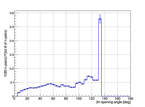
| + | The result of division of Y(80 n-pairs) over Y(tot # of n-pairs) is presented below | ||
| + | |||
| + | [[File:y80_over_ytot.png | 500px]] | ||
| + | |||
| + | ==Relative efficiency by random pairing neutrons from different pulses== | ||
| + | |||
| + | 2n opening angle distribution obtained by random sampling of neutron pairs (without repetition of a neutrons taken once) is presented below: | ||
| + | |||
| + | [[File:yuncorr_shuffle.png | 500px]] | ||
| + | |||
| + | The relative efficiency obtained as a result of division of 2n opening angle distribution in the case of correlated neutron pairs by 2n opening angle distribution obtained by random sampling of uncorrelated neutron pairs is presented below: | ||
| + | |||
| + | [[File:ycorr_over_yuncorr_shuffle.png | 500px ]] | ||
| + | |||
| + | ==Relative efficiency by pairing neutrons from different pulses (ascending event #)== | ||
| + | |||
| + | Another algorithm of neutron pairing was used to obtain the relative efficiency of the detecting system. Every run data file was sorted such that the event number order was ascending (see [https://wiki.iac.isu.edu/index.php/ASCII_data_files], second column in the table) and two neighboring neutrons from different detectors and different events were used to make a pair and the opening angle was calculated. | ||
| + | |||
| + | The normalization procedure of the opening angle distribution in the case of different pulses was the following | ||
| + | |||
| + | [[File:run_summary_norm.pdf]] | ||
| + | |||
| + | After going through the data one more time there were found some suspicious events. They were filtered out from the data. Now the range of 2n opening angles matches the range of the angles obtained via geant simulation for the current experimental setup (see the top section on the current page). | ||
| + | |||
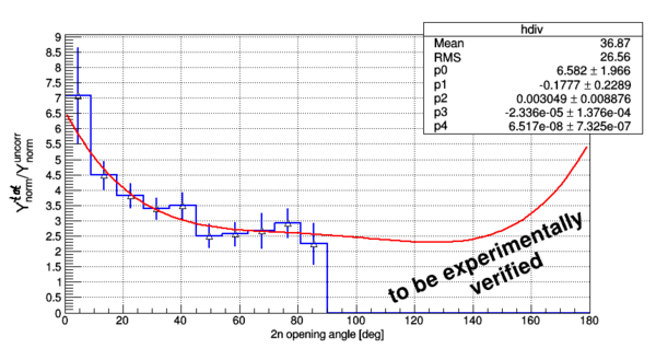
| + | The fit on the picture below shows one of the possible trends which the experimental data may follow and is needed to be experimentally proved. | ||
| + | |||
| + | Over the y-axis it is plotted normalized ratio <math>(Y^{corr}+Y^{uncorr})/Y^{uncorr} = Y^{tot}/Y^{uncorr}</math>. | ||
| + | |||
| + | [[File:Ycoor_ovr_Yuncorr_norm_cleaned3.png | 600px]] | ||
| + | |||
| + | ==The ratio of the integrated yields== | ||
| + | |||
| + | The ratio of the normalized integrated yields of correlated + uncorrelated neutrons per pulse <math>Y^{\text{tot}}=2.2E-5</math> and calculated yield of uncorrelated neutrons per pulse <math>Y^{\text{2n/fisson}}=6.49E-6</math> gives the following number <math>\frac{Y^{\text{tot}}}{Y^{\text{2 fisson}}}=3.4</math>. If we want to get the ratio of pure yield of correlated neutrons <math>Y^{\text{1n/fission}}</math> over the yield of uncorrelated neutrons <math>Y^{\text{2n/fisson}}</math> we should take the difference <math>Y^{\text{1n/fission}}=Y^{\text{tot}}-Y^{\text{2n/fisson}}</math> and then take the ratio <math>\frac{Y^{\text{1n/fission}}}{Y^{\text{2n/fisson}}} = \frac{(2.2E-5)-(6.49E-6)}{6.49E-6}=2.4</math> | ||
| + | |||
| + | Poisson distribution <math>P(n)=\frac{\bar{n}^n e^{-\bar{n}}}{n!}=\frac{(2.5)^ne^{-2.5}}{n!}</math> of the number of fission neutrons per fission event if the average number of neutrons emitted in fission event is 2.5 neutrons. | ||
| + | |||
| + | [[File:poisson_2_5n_ave.png | 500px]] | ||
| + | |||
| + | '''Bin-by-bin subtraction''' | ||
| + | |||
| + | |||
| + | Now let's plot the ratio <math>(Y^{tot}-Y^{uncorr})/Y^{uncorr}=Y^{corr}/Y^{uncorr}</math>. The error propagation is going to be the following: | ||
| + | |||
| + | <math>\frac{Y^{tot}-Y^{uncorr}}{Y^{uncorr}} = \frac{(a \pm \delta a) - (b \pm \delta b)}{(b \pm \delta b)}</math> | ||
| + | |||
| + | <math>=\frac{(a-b) \pm (\sqrt{\delta a^2 + \delta b^2})}{b \pm \delta b}</math> | ||
| + | |||
| + | <math>=\frac{a-b}{b} \pm Err(\frac{Y^{tot}-Y^{uncorr}}{Y^{uncorr}})</math> | ||
| + | |||
| + | <math>Err(\frac{Y^{tot}-Y^{uncorr}}{Y^{uncorr}}) = \frac{a-b}{b} \sqrt{\frac{\delta a^2 + \delta b^2}{(a-b)^2}+(\frac{\delta b}{b})^2}</math> | ||
| + | |||
| + | The plot of the ratio of yield of pure correlated neutrons over the yield of pure uncorrelated neutrons looks like | ||
| + | |||
| + | [[File:Pure_corrY_over_uncorrY2.png | 600px]] | ||
Latest revision as of 15:33, 22 September 2014
Some papers
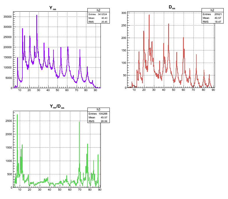
File:Nn correlation extraction.pdf
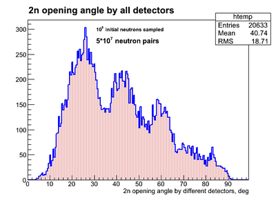
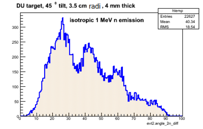
The result of simulation of 2n openeing angle obtained by different neutron detectors (each neutron hit different detector) having y-resolution is presented below. The source of neutrons was isotropic.
| Empty target, events sampled | DU target, events sampled |
|---|---|
|
|
| Point isotropic n-source w/o material | Volume isotropic n-source + DU material |
The result of simulation of 2n openeing angle obtained by the same neutron detectors (2 neutrons hit same detector) having y-resolution is presented below:
In the experiment our expereimental setup did not have y-resolution across the surface of the neutron detectors. So it was necessary to simulate the 2n opening angle for the neutron detectors w/o y-resolution. The result of the simulation of 2n opening angle (the 2n angles detected by all detectors are superimposed) for the case where thre was no y-resolution is going to be noted as . The experimental data obtained from run 4172 (DU target) on 2n opening angle for uncorrelated neutrons (i.e. in the case of isotropic source of neutrons) from different pulses is going to be noted as . The relative efficiency is defined as and it is plotted below as a result of bib-by-bin division of over .
Relative efficiency of the detecting system obtained using experimental data only (all runs)
In this part the experimantal data are presented for the cases when (1) the 2n opening angle was measured for neutrons correlated and (2) the 2n opening angle was measured for neutrons uncorrelated (neutrons from separate pulses). In the figure below the experimental data on the 2n opening angle measured for the case of correlated neutrons is presented where the statistical error bar width is equal to along y-axis and 4.5 deg along x-axis (the bin width). The total number of triggering pulses during the experiment was Nexp_pulses=2.469256E+7.
The experimental data on the 2n opening angle measured for the case of uncorrelated neutrons is presented in the next figure. 80 neutrons from different pulses were taken uniformly to reproduce 2n opening angle for the case of uncorrelated neutrons. The total number of uncorrelated neutron pairs was Npair_uncorr = 3.608397E+7. The width of the error bars is smaller then the size of the markers.
The result of the division of the two histograms () obtained for the described two cases is shown below. In order to obtain the resulting histogram as a division of the previous two histograms we need to do the division on the bin-by-bin basis as , where and are the contents of the corresponding bins and and are the coresponding statistical errors for the bin contents and . The error bars were obtained by the propagation in the following way: . The resulting histogram wa normalized to the ratio of the total number of pulses to the total number of uncorrelated neutron pairs considered Norm = Nexp_pulses/Npair_uncorr = 2.469256E+7/3.608397E+7 . It should be noted that the total number of uncorrelated neutron pairs can be varied by changing the number of corresponding combinations and the number of pulses involved into the 2n opening angle reproduction, so the normalization may change.
Normalization
Data table 1.
| run# | Total # of pulses per run |
|---|---|
| run4118 | 1668482 |
| run4119 | 2135901 |
| run4133 | 1704331 |
| run4134 | 1732490 |
| run4135 | 1603604 |
| run4137 | 800699 |
| run4144 | 1645667 |
| run4145 | 1544605 |
| run4146 | 510826 |
| run4153 | 1750657 |
| run4154 | 1631436 |
| run4155 | 1062048 |
| run4166 | 214600 |
| run4169 | 191592 |
| run4170 | 429974 |
| run4171 | 1141113 |
| run4172 | 650734 |
| run4173 | 354992 |
| run4174 | 953831 |
| run4175 | 299086 |
| run4176 | 144774 |
| run4177 | 225877 |
| run4203 | 659050 |
| run4204 | 1636192 |
| totals | 24692561 |
Normalization factor is 24692561.
Data table 2. Uncorrelated neutron pairs.
| run# | 80 puls pairs | all nonZ pairs | total # of pairs |
|---|---|---|---|
| run4118 | 1949796 | 35168980 | 58460510939894 |
| run4119 | 2470399 | 57115623 | 95803579611944 |
| run4133 | 1741760 | 30145143 | 60999663129029 |
| run4134 | 1832885 | 33384324 | 63031990015343 |
| run4135 | 1727993 | 28580648 | 54002495269034 |
| run4137 | 833189 | 7099684 | 13463513489481 |
| run4144 | 1770693 | 26603021 | 56872651957830 |
| run4145 | 1592222 | 20562899 | 50101929186175 |
| run4146 | 491705 | 2157292 | 5479817982802 |
| run4153 | 8753312 | 177560268 | 64360835399566 |
| run4154 | 1695297 | 26345381 | 55893286150871 |
| run4155 | 1182325 | 12257834 | 23686887361551 |
| run4166 | 174390 | 226636 | 967120869210 |
| run4169 | 175558 | 235498 | 770861409690 |
| run4170 | 319678 | 1008712 | 3882439488990 |
| run4171 | 1415700 | 19159461 | 27344940440490 |
| run4172 | 623978 | 3412116 | 8892563188751 |
| run4173 | 395573 | 1327163 | 2646413182232 |
| run4174 | 894440 | 5765727 | 19105685150123 |
| run4175 | 255450 | 619705 | 1878507428108 |
| run4176 | 110058 | 119818 | 440152774689 |
| run4177 | 976415 | 1721476 | 1071433552715 |
| run4203 | 3003073 | 23564022 | 9121298818219 |
| run4204 | 1682843 | 28829022 | 56219643867161 |
| totals | 36068732 | 542970453 | 734498220663898 |
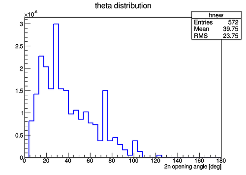
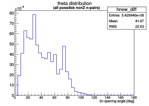
In the case if all possible non zero 2n pairs are considered the shape then the unncorrelated 2n opening angle distribution normalized looks like (the normalization factor is the total number of all possible n-pairs 734498220663898):
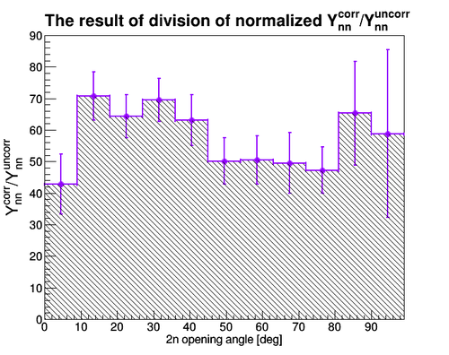
The division of normalized experimental data fir the case of correlared 2n pairs and uncorrelated 2n pairs (all non zero n pairs are taken into account) gives the following 2n angle distribution:
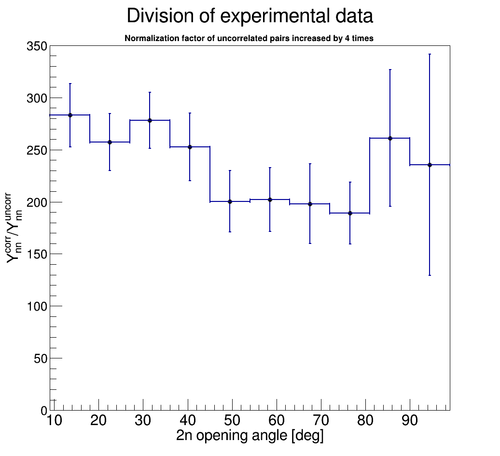
If the normalization factor of uncorrelated neutron pairs increased by 4 then the 2n opening angle distribution looks like:
Y(80 n-pairs)/Y(tot # of n-pairs)
| 80 uncorrelated neutron pairs uniformly distributed | All possible uncorrelated n-pairs |
|---|---|
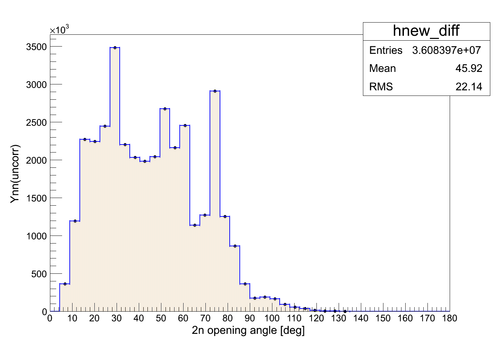
|
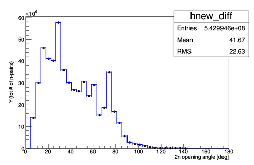
|
| 80 n-pairs algorithm | All possible combinations |
The result of division of Y(80 n-pairs) over Y(tot # of n-pairs) is presented below
Relative efficiency by random pairing neutrons from different pulses
2n opening angle distribution obtained by random sampling of neutron pairs (without repetition of a neutrons taken once) is presented below:
The relative efficiency obtained as a result of division of 2n opening angle distribution in the case of correlated neutron pairs by 2n opening angle distribution obtained by random sampling of uncorrelated neutron pairs is presented below:
Relative efficiency by pairing neutrons from different pulses (ascending event #)
Another algorithm of neutron pairing was used to obtain the relative efficiency of the detecting system. Every run data file was sorted such that the event number order was ascending (see [1], second column in the table) and two neighboring neutrons from different detectors and different events were used to make a pair and the opening angle was calculated.
The normalization procedure of the opening angle distribution in the case of different pulses was the following
After going through the data one more time there were found some suspicious events. They were filtered out from the data. Now the range of 2n opening angles matches the range of the angles obtained via geant simulation for the current experimental setup (see the top section on the current page).
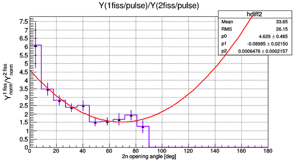
The fit on the picture below shows one of the possible trends which the experimental data may follow and is needed to be experimentally proved.
Over the y-axis it is plotted normalized ratio .
The ratio of the integrated yields
The ratio of the normalized integrated yields of correlated + uncorrelated neutrons per pulse and calculated yield of uncorrelated neutrons per pulse gives the following number . If we want to get the ratio of pure yield of correlated neutrons over the yield of uncorrelated neutrons we should take the difference and then take the ratio
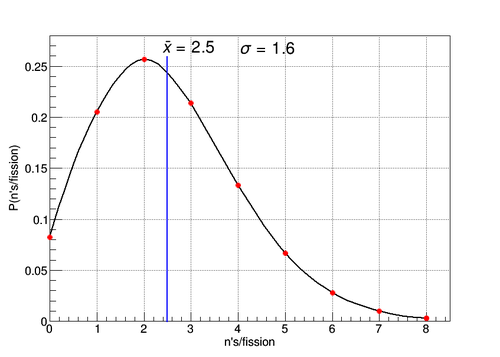
Poisson distribution of the number of fission neutrons per fission event if the average number of neutrons emitted in fission event is 2.5 neutrons.
Bin-by-bin subtraction
Now let's plot the ratio . The error propagation is going to be the following:
The plot of the ratio of yield of pure correlated neutrons over the yield of pure uncorrelated neutrons looks like
