Difference between revisions of "2n Position resolution"
| Line 102: | Line 102: | ||
{| cellpadding="2" style="border: 1px solid darkgray;" | {| cellpadding="2" style="border: 1px solid darkgray;" | ||
! width="400" | Fit: 6.7 cm/ns; Exp: 7.41 cm/ns | ! width="400" | Fit: 6.7 cm/ns; Exp: 7.41 cm/ns | ||
| − | ! width="400" | | + | ! width="400" | Fit: 5.7 cm/ns; Exp: 6.82 cm/ns |
! width="400" | Reconstructed | ! width="400" | Reconstructed | ||
|- border="0" | |- border="0" | ||
| Line 109: | Line 109: | ||
| [[File:resp_resol_DetF.png|400px|Region 3]] | | [[File:resp_resol_DetF.png|400px|Region 3]] | ||
|- align="center" | |- align="center" | ||
| − | | Res(fit) = 7 cm; Res(exp) = 7.7 cm|| | + | | Res(fit) = 7 cm; Res(exp) = 7.7 cm|| Res(fit) = 13.9 cm; Res(exp) = 16.6 cm||Fit: 5.8 cm/ns; Exp: 7.37 cm/ns |
|} | |} | ||
Revision as of 15:43, 10 May 2013
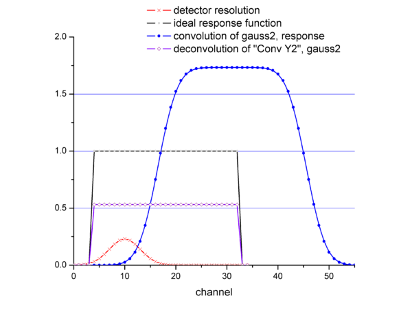
Discrete FFT algorithm test
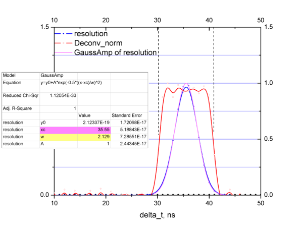
So as can be seen, deconvolution of the final curve (blue) with the resolution function (red) will give the response step function (black) which has the same shape as the initial step function.
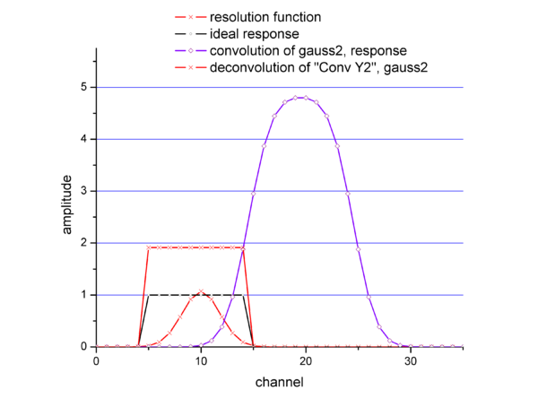
If we take narrower response function we will get
FFT application
In this section it was used run 4133 data with DU target.
Det G
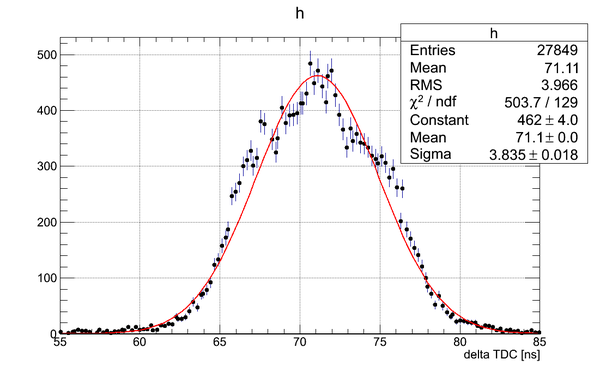
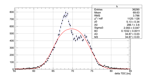
Experimental distribution of TDC difference time spectrum (black dots) and gaussian fit of the data (red line) are shown below:
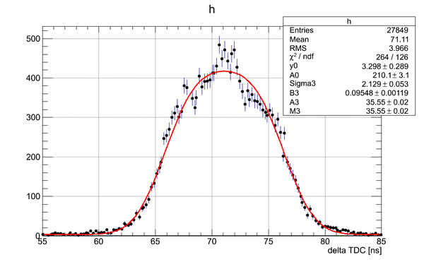
The fit of the experimental data with a function which is the result of convolution of the detector resolution function and detector response function is shown below
As can be seen the gaussian fit parameter "w" is equal to the parameter "Sigma3" of my_fcn fit of the experimental data and also "xc" is equal to "M3". Hence fitting the experimental data with my_fcn one can get the position resolution of the detector.
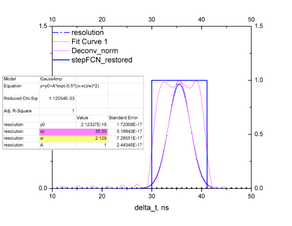
Comparison of the response function obtained as a result of the deconvolution of my_fit function and gaussian with the parameters from the fit and response function drawn using the parameters from the fit ("A3" and "B3").
The width of the ideal response function is 11 ns which corresponds to the result of the calibration with Co-60 source: for Det G (current case) it was obtained the conversion factor 7.24 cm/ns and, as the detector active area width is 75 cm, we obtain 75/7.24 = 10.36 ns width of the ideal response function.
Hence, any coordinate of the neutron hit has the following uncertainty in: sigma = 2.129 ns and its value converted into cm is 2.129 ns x 7.24 cm/ns = 15.4 cm. The total length of the active area of the neutron detector is 75 cm.
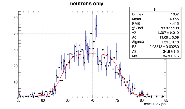
If we cut off all the photons from the distribution we will get:
In this case the position resolution is 1.59 ns x 7.24 cm/ns = 11.5 cm
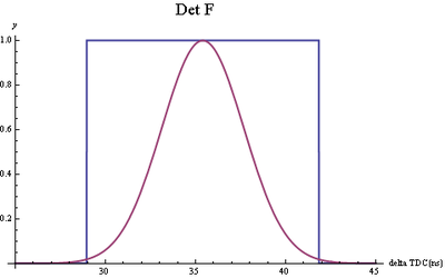
Det F
Fit of the experimental data in the case when photons and neutrons are combined:
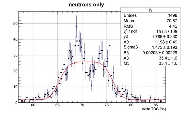
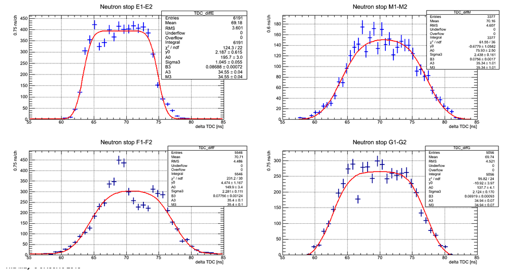
Fit of the experimental data in the case when only neutrons are included:
In this case the position resolution is 1.47 ns x 7.37 cm/ns = 10.8 cm
Det H
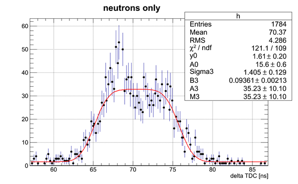
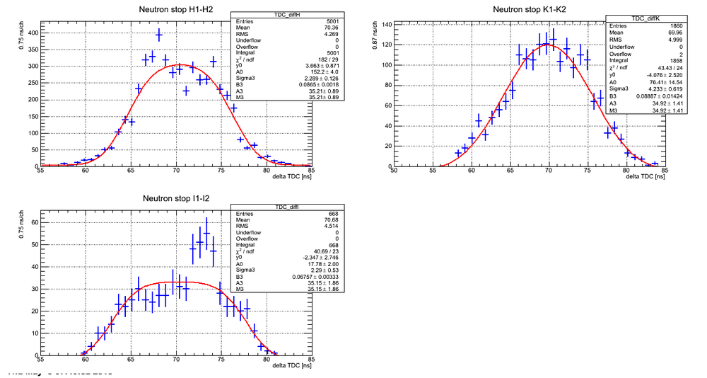
Fit of the experimental data in the case when only neutrons are included:
In this case the position resolution is 1.4 ns x 7.75 cm/ns = 10.85 cm
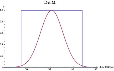
Det M
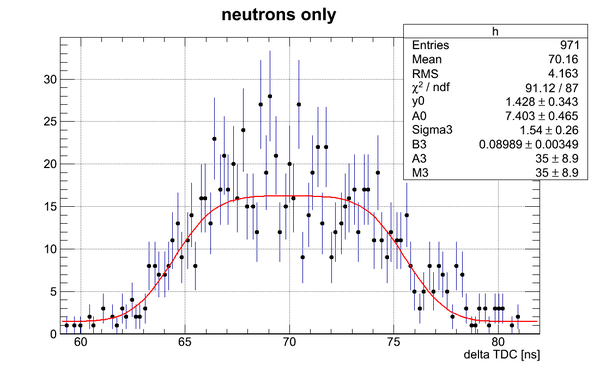
Fit of the experimental data in the case when only neutrons are included:
In this case the position resolution is 1.54 ns x 6.82 cm/ns = 10.5 cm
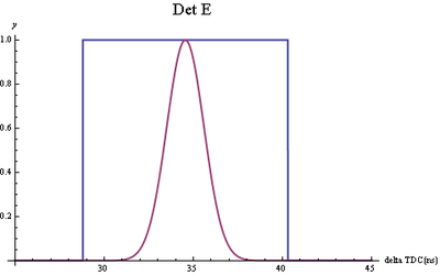
Det E
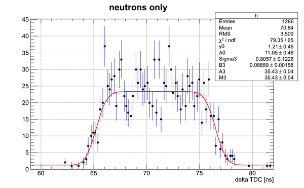
Fit of the experimental data in the case when only neutrons are included:
In this case the position resolution is 0.8 ns x 7.41 cm/ns = 5.9 cm
Det K
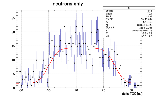
Fit of the experimental data in the case when only neutrons are included:
In this case the position resolution is 1.4 ns x 6.71 cm/ns = 9.4 cm
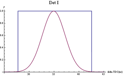
Det I
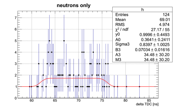
Fit of the experimental data in the case when only neutrons are included:
D2O data analysis
Response fcns and resolution fcns reconstructed
| Fit: 6.7 cm/ns; Exp: 7.41 cm/ns | Fit: 5.7 cm/ns; Exp: 6.82 cm/ns | Reconstructed |
|---|---|---|
|
|
|
| Res(fit) = 7 cm; Res(exp) = 7.7 cm | Res(fit) = 13.9 cm; Res(exp) = 16.6 cm | Fit: 5.8 cm/ns; Exp: 7.37 cm/ns |
| Reconstructed | Reconstructed | Reconstructed |
|---|---|---|
|
|
|
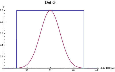
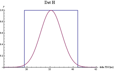
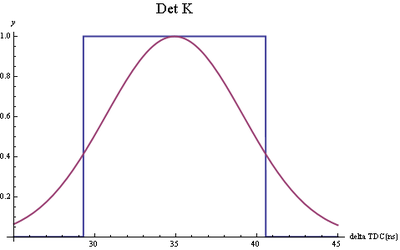
| Fit: 5.3 cm/ns; Exp: 7.24 cm/ns | Fit: 6.46 cm/ns; Exp: 7.75 cm/ns | Fit: 6.64 cm/ns; Exp: 6.71 cm/ns |
Fit: 5.1 cm/ns; Exp: 5.48 cm/ns
