Difference between revisions of "HRRL 03-18-2011"
| (35 intermediate revisions by 2 users not shown) | |||
| Line 119: | Line 119: | ||
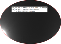
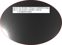
|[[File:HRRL_03-18-2011_cal_4_source.png | 200 px]] || [[File:HRRL_03-18-2011_cal_4.png | 200 px]] || cal_h = 31.75 mm / 735 px = 0.04320 mm/px; cal_v = 31.75 mm / sqrt(2) / 536 px = 0.04189 mm/px; | |[[File:HRRL_03-18-2011_cal_4_source.png | 200 px]] || [[File:HRRL_03-18-2011_cal_4.png | 200 px]] || cal_h = 31.75 mm / 735 px = 0.04320 mm/px; cal_v = 31.75 mm / sqrt(2) / 536 px = 0.04189 mm/px; | ||
|- | |- | ||
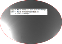
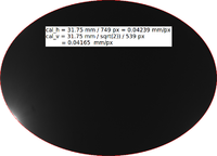
| + | |[[File:HRRL_03-18-2011_cal_5_source.png | 200 px]] || [[File:HRRL_03-18-2011_cal_5.png | 200 px]] || cal_h = 31.75 mm / 749 px = 0.04239 mm/px; cal_v = 31.75 mm / sqrt(2)) / 539 px = 0.04165 mm/px | ||
| + | |- | ||
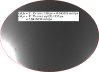
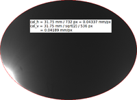
| + | |[[File:HRRL_03-18-2011_cal_6_source.png | 200 px]] || [[File:HRRL_03-18-2011_cal_6.png | 200 px]] || cal_h = 31.75 mm / 732 px = 0.04337 mm/px; cal_v = 31.75 mm / sqrt(2) / 536 px = 0.04189 mm/px | ||
| + | |- | ||
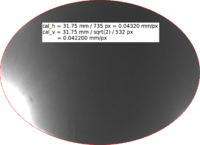
| + | |[[File:HRRL_03-18-2011_cal_7_source.png | 200 px]] || [[File:HRRL_03-18-2011_cal_7.png | 200 px]] || cal_h = 31.75 mm / 735 px = 0.04320 mm/px; cal_v = 31.75 mm / sqrt(2)) / 532 px = 0.04220 mm/px | ||
| + | |- | ||
| + | |} | ||
| + | |||
| + | {| border="3" cellpadding="20" cellspacing="0" | ||
| + | |- | ||
| + | |cal_h (mm/px) || cal_v (mm/px) || | ||
| + | |- | ||
| + | |0.04308|| 0.04228 || | ||
| + | |- | ||
| + | |0.04302 || 0.04196 || | ||
| + | |- | ||
| + | |0.04320 || 0.04220 || | ||
| + | |- | ||
| + | |0.04320 || 0.04189 || | ||
| + | |- | ||
| + | |0.04239 || 0.04165 || | ||
| + | |- | ||
| + | |0.04337 || 0.04189 || | ||
| + | |- | ||
| + | |0.04320 || 0.04220 || | ||
| + | |- | ||
| + | | mean (mm/px) || mean (mm/px) || | ||
| + | |- | ||
| + | | <math> 0.04307 \pm 0.00032 </math>|| <math> 0.04201 \pm 0.00023 </math> || | ||
|} | |} | ||
| Line 147: | Line 176: | ||
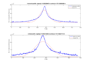
Fitted Gaussian for whole image | Fitted Gaussian for whole image | ||
x-projection: | x-projection: | ||
| − | |||
| − | |||
| − | |||
| − | |||
[[File:HRRL_03-18-2011_Data_Analysis_Preliminary_Results_Gauss_Fitted_Whole_Image.png | 300 px]] | [[File:HRRL_03-18-2011_Data_Analysis_Preliminary_Results_Gauss_Fitted_Whole_Image.png | 300 px]] | ||
| Line 168: | Line 193: | ||
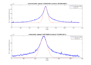
x-projection: | x-projection: | ||
| − | |||
| − | |||
| − | |||
[[File:HRRL_03-18-2011_Data_Analysis_Preliminary_Results_Gauss_Fitted_Part_1_Image.png | 300 px]] | [[File:HRRL_03-18-2011_Data_Analysis_Preliminary_Results_Gauss_Fitted_Part_1_Image.png | 300 px]] | ||
| − | |||
=== Gaussian fitted for part 2 of the image === | === Gaussian fitted for part 2 of the image === | ||
| Line 186: | Line 207: | ||
x-projection: | x-projection: | ||
| − | |||
| − | |||
| − | |||
| − | |||
| Line 205: | Line 222: | ||
x-projection: | x-projection: | ||
| − | |||
| − | |||
| − | |||
| − | |||
| Line 226: | Line 239: | ||
x-projection: | x-projection: | ||
| − | |||
| − | |||
| − | |||
[[File:HRRL_03-18-2011_Data_Analysis_Preliminary_Results_Gauss_Fitted_Part_4_Image.png | 300 px]] | [[File:HRRL_03-18-2011_Data_Analysis_Preliminary_Results_Gauss_Fitted_Part_4_Image.png | 300 px]] | ||
| Line 291: | Line 301: | ||
|} | |} | ||
| + | |||
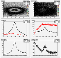
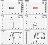
| + | [[File:TF_Q1_1.8_03182011_NOCUTS.png| 200 px]][[File:TF_Q1_1.8_03182011.png| 200 px]] | ||
| + | |||
| + | The red line is the background above which seems to be larger than the signal. Why? | ||
| + | |||
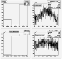
| + | Below I zoom in on channel 250 where you can see that for this channel the background is larger. I then plot, on the right, all the elements along the x direction what are added up to get the values on the right. | ||
| + | |||
| + | [[File:TF_Q1_1.8_03182011Problem.png| 200 px]] | ||
| + | |||
| + | Why isn't the addition making sense? | ||
=== Q6_Scan, 42mA peak current, Scan Coil Current at negative 2.5_Amp === | === Q6_Scan, 42mA peak current, Scan Coil Current at negative 2.5_Amp === | ||
| Line 309: | Line 329: | ||
|} | |} | ||
| + | |||
| + | [[File:TF_Q6_2.5_03182011.png| 200px]] | ||
== Lorentzian Fitting == | == Lorentzian Fitting == | ||
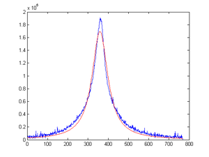
| Line 335: | Line 357: | ||
| 1.6935e+006 || 358.9910 || 45.4280 | | 1.6935e+006 || 358.9910 || 45.4280 | ||
|} | |} | ||
| + | |||
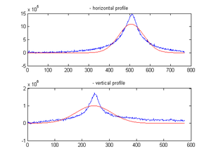
| + | If we were to apply the relation of the Gaussian rms to its FWHM to Lorentzian, we will get the sigma (or rms) of Lorentzian to be: | ||
| + | <math> \frac {2 \times 45.4280}{ 2.3548} = 38.5833192 </math> | ||
| + | |||
| + | |||
| + | == Super Gaussian Fitting == | ||
| + | |||
| + | Beam Distributions Beyond RMS: | ||
| + | [[File:Beam_Distributions_Beyond_RMS.pdf]] | ||
| + | |||
| + | Bib: http://www.osti.gov/bridge/product.biblio.jsp?osti_id=82539# | ||
| + | |||
| + | |||
| + | Basic MATLAB Codes to fit Super Gaussian: | ||
| + | |||
| + | [[File:Trial_my_Super_Gaussian_fit.txt]] | ||
| + | |||
| + | [[File:SupGau_desum.txt]] | ||
| + | |||
| + | My MATLAB Fit code for beam | ||
| + | |||
| + | [[File:my_Super_Gaussian_fit.txt]] | ||
| + | |||
| + | [[File:SupGau_desum.txt]] | ||
| + | |||
| + | Here is an example fitting: | ||
| + | |||
| + | {| border="1" | ||
| + | | Signal || Background || fit | ||
| + | |- | ||
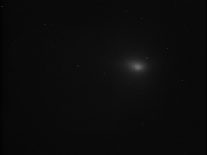
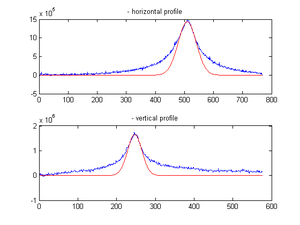
| + | | [[File:HRRL_03-18-2011_Lorentzian_Fitting_Example_sg.png| 300 px]] || [[File:HRRL_03-18-2011_Lorentzian_Fitting_Example_bg.png| 300 px]] || [[File:HRRL_03-18-2011_SupGau_Fitting_Example_1.png| 300 px]] | ||
| + | |||
| + | |||
| + | |||
| + | [[HRRL_Emittance_Measurements_March14-18-2011]] | ||
| + | |||
| + | |- | ||
| + | | base || Amplitude || center | ||
| + | |- | ||
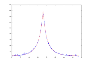
| + | | 202 || 8.0480e+003 || 359.6730 | ||
| + | |- | ||
| + | | sigma_0 || N || sigma | ||
| + | |- | ||
| + | | 20.92 || 0.8494 || 38.56 | ||
| + | |} | ||
| + | |||
| + | |||
| + | If we were to apply the relation of the Gaussian rms to its FWHM to Lorentzian, we will get the sigma (or rms) of Lorentzian to be: | ||
| + | <math> \frac {2 \times 45.4280}{ 2.3548} = 38.5833192 </math> | ||
| + | |||
| + | This is very close to the sigma we got from Super Gaussian, which is 38.56 | ||
| + | |||
| + | = Results = | ||
| + | |||
| + | == Q1 == | ||
| + | |||
| + | === Positive Current, X projection === | ||
| + | |||
| + | ==== 1st fit ==== | ||
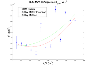
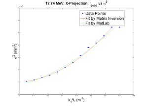
| + | [[File:HRRL 03-18-2011_Results_Q1_42mA_Pos_X.png | 300 px]] | ||
| + | ==== 2nd fit after cut off some points ==== | ||
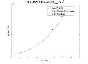
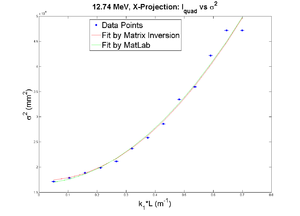
| + | [[File:HRRL 03-18-2011_Results_Q1_42mA_Pos_X_2.png | 300 px]] | ||
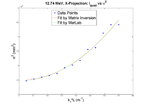
| + | == Q4 == | ||
| + | Did not reach minimum. | ||
Latest revision as of 19:13, 11 January 2012
Tune parameters
Previous Tune at the higher energy
| Solenoid 1 | 5.4 A |
| Solenoid 2 | 5.5 A |
| Gun Ver | -0.2 A |
| Gun Hor | +0.4 A |
| Output Hor | -0.5 A |
| Output Ver | -0.5 A |
| Gun HV | +9.75 (Knob Setting) |
| Gun Grid Voltage | 5.25 (Knob Setting) |
| RF frequency | 2855.813 MHz |
| Modulator HV Power Supply | 4.11 (Knob Setting) |
| RF macro Pulse Length (FWHM) | 200 ns |
Solenoid comparison with yesterdays higher energy tune
Quad Scans
To test reproducibility from yesterday. Scan at 40, 20, 10, 5 mA peak currents. Scan twice on each Current.
Do Energy Scan
Bend the beam through 45 bending dipole, take images on the scope of FC and YAG images.
| D1 current | Energy | FC peak Volt | Pic |
| (A) | MeV | mV | |
| 28 | 11.85 | 39 | 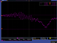
|
| 29 | 12.3 | 74 | 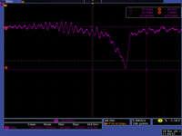
|
| 30 | 12.74 | 93 | 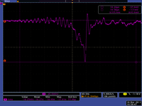
|
| 30.5 | 12.96 | 65 | 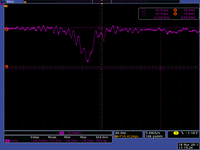
|
| 30.7 | large uncertainty | 22 | 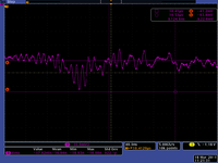
|
Quad 1 Scan
| Quad 1 | OTR Pict | FC pict |
| (A) | ||
| +0 |  |

|
| +0.2 |  |

|
| +0.4 |  |

|
| +0.6 |  |

|
| +0.8 |  |

|
| +1.0 |  |

|
| +1.2 |  |

|
| +1.4 |  |

|
| +1.6 |  |

|
| +1.8 |  |

|
| +2.0 |  |

|
Scan Quad 4
Calibration
Estimate the error in the above calibration
| cal_h (mm/px) | cal_v (mm/px) | |
| 0.04308 | 0.04228 | |
| 0.04302 | 0.04196 | |
| 0.04320 | 0.04220 | |
| 0.04320 | 0.04189 | |
| 0.04239 | 0.04165 | |
| 0.04337 | 0.04189 | |
| 0.04320 | 0.04220 | |
| mean (mm/px) | mean (mm/px) | |
Data Analysis
Preliminary results
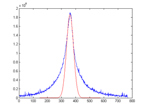
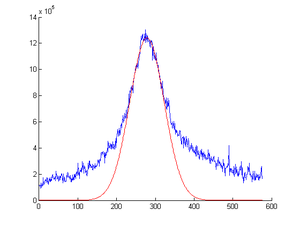
Here is the study on how to fit non_Gaussian curve. I fitted for whole image as well as parts of the image.
Here is beam profile, which is non-Gaussian.
Fits for whole image:
Fits for x=[362,404] and y=[241,301]:
Gaussian fitted for whole image
12.74 MeV
Fitted Gaussian for whole image x-projection:
Gaussian fitted for part 1 of the image
Fitted Gaussian for part 1 of the image
       xl = 362;% center at 382
       xr = 404;
       yl = 241;% center at 271
       yr = 301;
xl: x left, xr: x right. yl: y left, yr: y right.
x-projection:
Gaussian fitted for part 2 of the image
Fitted Gaussian for part 2 of the image
       xl = 342;% center at 382
       xr = 424;
       yl = 241;% center at 271
       yr = 301;
x-projection:
Gaussian fitted for part 3 of the image
Fitted Gaussian for part 3 of the image
       xl = 342;% center at 382
       xr = 424;
       yl = 221;% center at 271
       yr = 321;
x-projection:
Gaussian fitted for part 4 of the image
Fitted Gaussian for part 4 of the image
       xl = 322;% center at 382
       xr = 444;
       yl = 221;% center at 271
       yr = 321;
x-projection:
Analysis with root
Q1_Scan, 42mA peak current, Scan Coil Current at positive 1.8_Amp
Back grounds
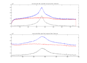
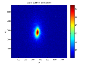
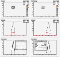
The red line is the background above which seems to be larger than the signal. Why?
Below I zoom in on channel 250 where you can see that for this channel the background is larger. I then plot, on the right, all the elements along the x direction what are added up to get the values on the right.
Why isn't the addition making sense?
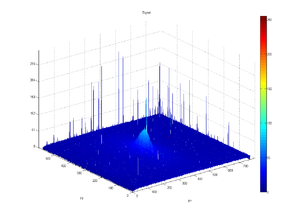
Q6_Scan, 42mA peak current, Scan Coil Current at negative 2.5_Amp
Lorentzian Fitting
Basic MATLAB Codes to fit Lorentzian:
File:Trial my Lorentzian fit.txt
My MATLAB Fit code for beam
Here is an example fitting:
| Signal | Background | fit |
 |
 |
|
| height of the peak | location of the peak | half-width at half-maximum (HWHM) |
| 1.6935e+006 | 358.9910 | 45.4280 |
If we were to apply the relation of the Gaussian rms to its FWHM to Lorentzian, we will get the sigma (or rms) of Lorentzian to be:
Super Gaussian Fitting
Beam Distributions Beyond RMS: File:Beam Distributions Beyond RMS.pdf
Bib: http://www.osti.gov/bridge/product.biblio.jsp?osti_id=82539#
Basic MATLAB Codes to fit Super Gaussian:
File:Trial my Super Gaussian fit.txt
My MATLAB Fit code for beam
File:My Super Gaussian fit.txt
Here is an example fitting:
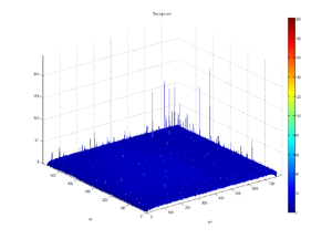
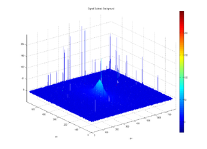
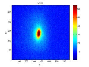
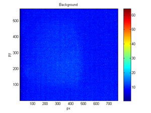
| Signal | Background | fit |
 |
 |
|
| base | Amplitude | center |
| 202 | 8.0480e+003 | 359.6730 |
| sigma_0 | N | sigma |
| 20.92 | 0.8494 | 38.56 |
If we were to apply the relation of the Gaussian rms to its FWHM to Lorentzian, we will get the sigma (or rms) of Lorentzian to be:
This is very close to the sigma we got from Super Gaussian, which is 38.56
Results
Q1
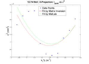
Positive Current, X projection
1st fit
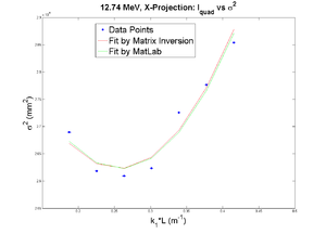
2nd fit after cut off some points
Q4
Did not reach minimum.


