Difference between revisions of "Lab 13 RS"
| (17 intermediate revisions by the same user not shown) | |||
| Line 88: | Line 88: | ||
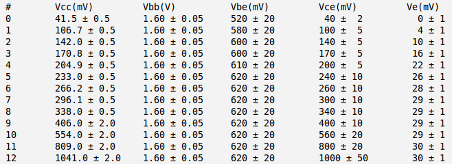
Below is the table with my measurements: | Below is the table with my measurements: | ||
| − | [[File:Table 2uA 01.png | | + | [[File:Table 2uA 01 corrected.png | 700 px]] |
| Line 94: | Line 94: | ||
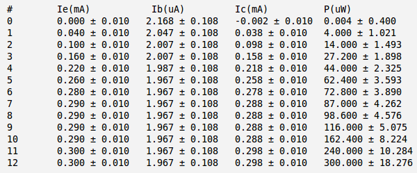
Here: | Here: | ||
| + | |||
<math>I_{E} = \frac{V_E}{R_E}</math> | <math>I_{E} = \frac{V_E}{R_E}</math> | ||
| − | <math>I_{B} | + | <math>I_{B} \approx \frac{V_{BB}-V_{BE}}{R_B}</math> |
| − | <math>P_{max} = I_C \cdot V_{ | + | <math>P_{max} = I_C \cdot V_{CE} = (I_E - I_B) \cdot V_{CE} </math> |
| + | |||
| + | and I have used approximation <math>V_{E} \approx o</math> | ||
| + | |||
| − | [[File:Table 2uA 02.png | | + | [[File:Table 2uA 02 corrected.png | 700 px]] |
| Line 112: | Line 116: | ||
Below is the table with my measurements: | Below is the table with my measurements: | ||
| − | [[File:Table 5uA 01.png | | + | [[File:Table 5uA 01 corrected.png | 700 px]] |
| Line 118: | Line 122: | ||
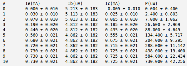
Here: | Here: | ||
| + | |||
<math>I_{E} = \frac{V_E}{R_E}</math> | <math>I_{E} = \frac{V_E}{R_E}</math> | ||
| − | <math>I_{B} | + | <math>I_{B} \approx \frac{V_{BB}-V_{BE}}{R_B}</math> |
| − | <math>P_{max} = I_C \cdot V_{ | + | <math>P_{max} = I_C \cdot V_{CE} = (I_E - I_B) \cdot V_{CE} </math> |
| + | |||
| + | and I have used approximation <math>V_{E} \approx o</math> | ||
| + | |||
| − | [[File:Table 5uA 02.png | | + | [[File:Table 5uA 02 corrected.png | 700 px]] |
| Line 138: | Line 146: | ||
Below is the table with my measurements: | Below is the table with my measurements: | ||
| − | [[File:Table 10uA 01.png | | + | [[File:Table 10uA 01 corrected.png | 700 px]] |
| Line 144: | Line 152: | ||
Here: | Here: | ||
| + | |||
<math>I_{E} = \frac{V_E}{R_E}</math> | <math>I_{E} = \frac{V_E}{R_E}</math> | ||
| − | <math>I_{B} | + | <math>I_{B} \approx \frac{V_{BB}-V_{BE}}{R_B}</math> |
| − | <math>P_{max} = I_C \cdot V_{ | + | <math>P_{max} = I_C \cdot V_{CE} = (I_E - I_B) \cdot V_{CE} </math> |
| + | |||
| + | and I have used approximation <math>V_{E} \approx o</math> | ||
| + | |||
| − | [[File:Table 10uA 02.png | | + | [[File:Table 10uA 02 corrected.png | 700 px]] |
| Line 171: | Line 183: | ||
| − | + | ||
'''6.) Overlay points from the transistor's data sheet on the graph in part 5.).(10 pnts)''' | '''6.) Overlay points from the transistor's data sheet on the graph in part 5.).(10 pnts)''' | ||
| Line 180: | Line 192: | ||
And from the table above I can only extract the range of <math>I_B</math> like | And from the table above I can only extract the range of <math>I_B</math> like | ||
| − | 1) <math>I_C = 0.1\ mA,\ V_{CE} = 1.0\ V \rightarrow I_B = \frac{I_C}{ | + | 1) <math>I_C = 0.1\ mA,\ V_{CE} = 1.0\ V \rightarrow I_B = \frac{I_C}{\beta} = \frac{0.1}{40..300} = (2.5 - 0.33)\ \mu A</math> |
| − | 2) <math>I_C = 1.0\ mA,\ V_{CE} = 1.0\ V \rightarrow I_B = \frac{I_C}{ | + | 2) <math>I_C = 1.0\ mA,\ V_{CE} = 1.0\ V \rightarrow I_B = \frac{I_C}{\beta} = \frac{0.1}{70..300} = (14.2 - 3.3)\ \mu A</math> |
And my measurements looks like: | And my measurements looks like: | ||
| Line 192: | Line 204: | ||
3) <math>I_B = 10\ \mu A,\ I_C = 1.40\ mA,\ V_{CE} = 1.0\ V \rightarrow \beta = \frac{I_C}{I_B} = \frac{1.40\ mA}{10\ uA} = 140</math> | 3) <math>I_B = 10\ \mu A,\ I_C = 1.40\ mA,\ V_{CE} = 1.0\ V \rightarrow \beta = \frac{I_C}{I_B} = \frac{1.40\ mA}{10\ uA} = 140</math> | ||
| − | First point to note that <math>I_C</math> from my measurements and from data sheet are different so I can not really | + | First point to note that <math>I_C</math> from my measurements and from data sheet are different so I can not really overlay them and compare. |
Second, I have specific values of <math>I_B</math>, otherwise from data sheet I have the range of <math>I_B</math>. | Second, I have specific values of <math>I_B</math>, otherwise from data sheet I have the range of <math>I_B</math>. | ||
And third, I can't really plot this range of <math>I_B</math> from data sheet on my plots just because my plot doesn't have the <math>I_B</math> axis. | And third, I can't really plot this range of <math>I_B</math> from data sheet on my plots just because my plot doesn't have the <math>I_B</math> axis. | ||
| − | All I can do here is to say that my measured <math>\beta</math> | + | All I can do here is to say that my measured <math>\beta</math> are inside the range of data sheet <math>\beta</math>. |
=Questions= | =Questions= | ||
| Line 220: | Line 232: | ||
3) The base must always be more <u>positive</u> (<u>negative</u>) than the emitter for a npn (pnp) transistor to conduct I_C.(10 pnts) | 3) The base must always be more <u>positive</u> (<u>negative</u>) than the emitter for a npn (pnp) transistor to conduct I_C.(10 pnts) | ||
| − | 4) For a transistor to conduct I_{C} the base-emitter junction must be <u>forward</u> biased.(10 pnts) | + | 4) For a transistor to conduct <math>I_{C}</math> the base-emitter junction must be <u>forward</u> biased.(10 pnts) |
| − | 5) For a transistor to conduct I_{C} the collector-base junction must be <u>reversed</u> biased.(10 pnts) | + | 5) For a transistor to conduct <math>I_{C}</math> the collector-base junction must be <u>reversed</u> biased.(10 pnts) |
=Extra credit= | =Extra credit= | ||
| Line 241: | Line 253: | ||
Below is the table with my measurements and current calculations: | Below is the table with my measurements and current calculations: | ||
| − | Here: | + | Here I have used exact formula to calculate <math>I_B</math>: |
| + | |||
<math>I_{B} = \frac{V_{BB}-V_B}{R_B}</math> | <math>I_{B} = \frac{V_{BB}-V_B}{R_B}</math> | ||
| Line 251: | Line 264: | ||
[[File:Plot extra fitted.png | 1000 px ]] | [[File:Plot extra fitted.png | 1000 px ]] | ||
| − | |||
| − | <math>V_{BE} = \frac{p_0}{p_1} = \frac{111.7 \pm 10.61}{0.1809 \pm 0.01634} = (617.46 \pm 80.93) | + | The fitting line is <math>I_B\ (\mu A) = (111.7 \pm 10.61) + (0.1809 \pm 0.01634)\ (mV) </math>. The intersection this line with x-axis gives the forward turn on voltage: |
| + | |||
| + | <math>V_{BE} = \frac{p_0}{p_1} = \frac{111.7 \pm 10.61}{0.1809 \pm 0.01634} = (617.46 \pm 80.93)\ mV</math> | ||
| − | Actually what we are measuring here is better to call the forward turn on voltage for base-emitter junction (Base-Emitter breakdown voltage is for reverse current measurement). From the data sheet this point (called the base-emitter saturation voltage) is 0.65 V and this point is inside my predicted values <math>(617.46 \pm 80.93) | + | Actually what we are measuring here is better to call the forward turn on voltage for base-emitter junction (Base-Emitter breakdown voltage is for reverse current measurement). From the data sheet this point (called the base-emitter saturation voltage) is 0.65 V and this point is inside my predicted values <math>(617.46 \pm 80.93)\ mV</math> |
[https://wiki.iac.isu.edu/index.php/Electronics_RS Go Back to All Lab Reports] [[Forest_Electronic_Instrumentation_and_Measurement]] | [https://wiki.iac.isu.edu/index.php/Electronics_RS Go Back to All Lab Reports] [[Forest_Electronic_Instrumentation_and_Measurement]] | ||
Latest revision as of 04:07, 22 March 2011
DC Bipolar Transistor Curves
Data sheet for transistors.
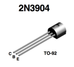
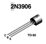
Media:2N3904.pdf Media:2N3906.pdf
Using 2N3904 is more srtaight forward in this lab.
Transistor circuit
1.) Identify the type (n-p-n or p-n-p) of transistor you are using and fill in the following specifications.
I am going to use n-p-n transistor 2N3904. Below are some specifications from data shits for this type of transistor:
| Value | Description | ||
|---|---|---|---|
| Collector-Base breakdown voltage | |||
| Emitter-Base Breakdown Voltage | |||
| Maximum Collector-Emitter Voltage | |||
| Maximum Collector-Emitter Voltage | |||
| Maximum Collector Current - Continuous | |||
| Transistor Power rating() | |||
| , | |||
| 40 | 300 | , | |
| 70 | 300 | , | |
| 100 | 300 | , | |
| 60 | 300 | , | |
| 30 | 300 | , | |
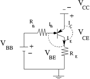
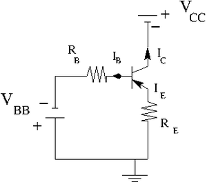
2.) Construct the circuit below according to the type of transistor you have.
Let .
variable power supply
.
Find the resistors you need to have
, , and
By measurements I was able to find that . So I am going to use this value. Also let picks up . So my current .
Now to get I need to use To get I need to use To get I need to use
3.) Measure the emitter current for several values of by changing such that the base current A is constant.
I used:
and
Below is the table with my measurements:
And below is my currents and power calculation:
Here:
and I have used approximation
4a.) Repeat the previous measurements for . Remember to keep so the transistor doesn't burn out
I used:
and
Below is the table with my measurements:
And below is my currents and power calculation:
Here:
and I have used approximation
4a.) Repeat the previous measurements for . Remember to keep so the transistor doesn't burn out
I used:
and
Below is the table with my measurements:
And below is my currents and power calculation:
Here:
and I have used approximation
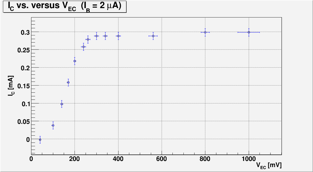
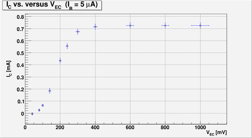
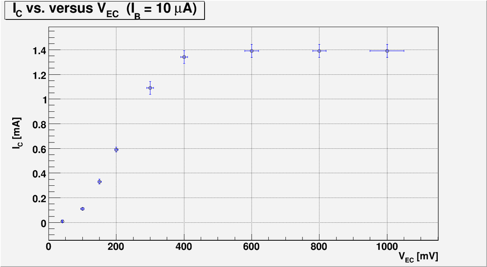
5.) Graph -vs- for each value of and above. (40 pnts)
Bellow is my plot for the case of
Bellow is my plot for the case of
Bellow is my plot for the case of
6.) Overlay points from the transistor's data sheet on the graph in part 5.).(10 pnts)
I can not really do it because there are not good points to compare from data sheet. I can take for example this data from data sheet:
And from the table above I can only extract the range of like
1)
2)
And my measurements looks like:
1)
2)
3)
First point to note that from my measurements and from data sheet are different so I can not really overlay them and compare. Second, I have specific values of , otherwise from data sheet I have the range of . And third, I can't really plot this range of from data sheet on my plots just because my plot doesn't have the axis.
All I can do here is to say that my measured are inside the range of data sheet .
Questions
1) Compare your measured value of or for the transistor to the spec sheet? (10 pnts)
I will calculate my from my measurements above in active region like:
1):
2):
3):
And above values of are in agreement with range of from the spec sheet which is from 30 to 300. But I can not say nothing more because 1) my current doesn't correspond to published in data sheet. 2) My calculation is for specific value of current. But in the data sheet the range of is reported for specific values of and .
2) What is for the transistor? (10 pnts)
3) The base must always be more positive (negative) than the emitter for a npn (pnp) transistor to conduct I_C.(10 pnts)
4) For a transistor to conduct the base-emitter junction must be forward biased.(10 pnts)
5) For a transistor to conduct the collector-base junction must be reversed biased.(10 pnts)
Extra credit
Measure the Base-Emitter breakdown voltage. (10 pnts)
I expect to see a graph and a linear fit which is similar to the forward biased diode curves. Compare your result to what is reported in the data sheet.
I used:
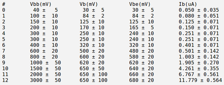
Below is the table with my measurements and current calculations:
Here I have used exact formula to calculate :
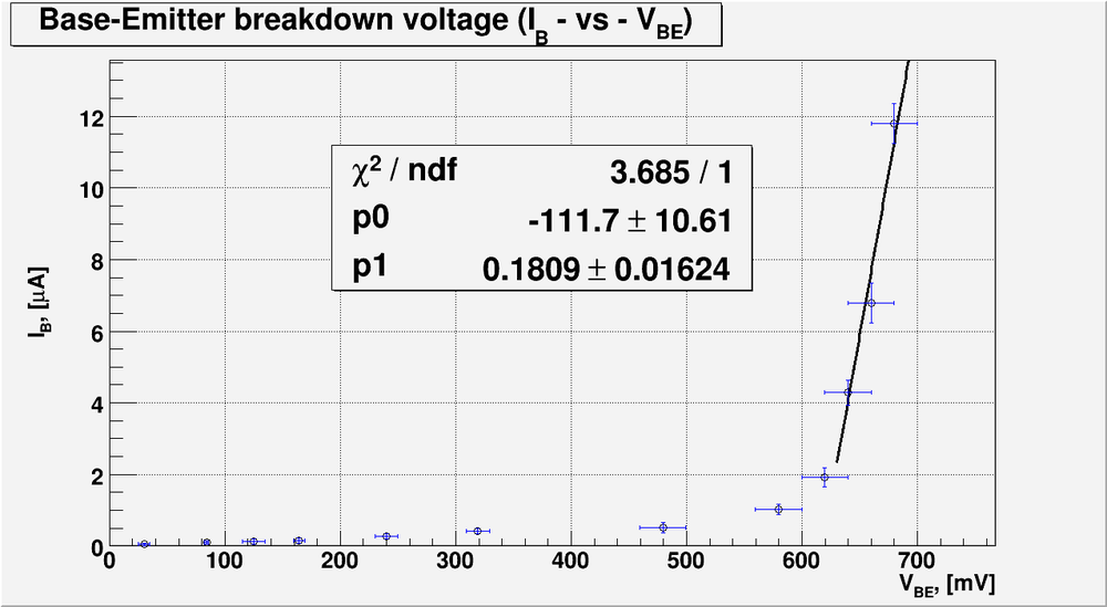
And bellow is my plot for the Base-Emitter breakdown voltage
The fitting line is . The intersection this line with x-axis gives the forward turn on voltage:
Actually what we are measuring here is better to call the forward turn on voltage for base-emitter junction (Base-Emitter breakdown voltage is for reverse current measurement). From the data sheet this point (called the base-emitter saturation voltage) is 0.65 V and this point is inside my predicted values
Go Back to All Lab Reports Forest_Electronic_Instrumentation_and_Measurement
