Difference between revisions of "Tamar AnalysisChapt"
| Line 1: | Line 1: | ||
| − | |||
=Introduction= | =Introduction= | ||
| Line 7: | Line 6: | ||
There are couple of main steps in the data analysis, which will be discussed bellow: 1) the data selection, 2) background elimination, 3) the target and beam polarization, 4) the detector acceptance >??????? | There are couple of main steps in the data analysis, which will be discussed bellow: 1) the data selection, 2) background elimination, 3) the target and beam polarization, 4) the detector acceptance >??????? | ||
| + | =Beam Helicity and Charge Asymmetry= | ||
| + | |||
| + | In double spin asymmetry measurements it is important to eliminate any source of false asymmetry, like charge asymmetry. | ||
| + | |||
| + | The helicity of the electron beam was flipped with a rate of 1 HZ and its original state was chosen at the injector in a pseudo-random way. The next state of the electron helicity, so called complement state, is always with opposite helicity. The diagram on Fig.?.? represents the helicity state. | ||
| + | |||
| + | '''Figure ??. The Helicity State''' | ||
| + | |||
| + | A one bit signal from the beam injector gives the helicity information, whereas a sync bit with a 2 HZ frequency is generated at the same time and is equal to the helicity flip time. However, the electron beam helicity sequence can be interrupted by the Data Acquisition System(DAQ), like leaving unpaired helicity states and dead time problems. | ||
| + | |||
| + | In order to eliminate the asymmetry caused by the DAQ, the Faraday cup was installed to measure the charge simultaneously with the helicity state flip. The stored data files include accumulated charge value for each helicity state. | ||
| + | |||
| + | =Data Analysis= | ||
==Radiative Corrections== | ==Radiative Corrections== | ||
Revision as of 20:23, 7 February 2011
Introduction
THIS CHAPTER IS NOT READY< PLEASE READ OTHER THREE CHAPTERS.
This chapter will describe the techniques to calculate semi inclusive double spin asymmetries for the following reactions and for NH3 and ND3 polarized targets respectively. The goal of this work is the extraction of the ratio of polarized to unpolarized quark distribution functions using double spin asymmetries.
There are couple of main steps in the data analysis, which will be discussed bellow: 1) the data selection, 2) background elimination, 3) the target and beam polarization, 4) the detector acceptance >???????
Beam Helicity and Charge Asymmetry
In double spin asymmetry measurements it is important to eliminate any source of false asymmetry, like charge asymmetry.
The helicity of the electron beam was flipped with a rate of 1 HZ and its original state was chosen at the injector in a pseudo-random way. The next state of the electron helicity, so called complement state, is always with opposite helicity. The diagram on Fig.?.? represents the helicity state.
Figure ??. The Helicity State
A one bit signal from the beam injector gives the helicity information, whereas a sync bit with a 2 HZ frequency is generated at the same time and is equal to the helicity flip time. However, the electron beam helicity sequence can be interrupted by the Data Acquisition System(DAQ), like leaving unpaired helicity states and dead time problems.
In order to eliminate the asymmetry caused by the DAQ, the Faraday cup was installed to measure the charge simultaneously with the helicity state flip. The stored data files include accumulated charge value for each helicity state.
Data Analysis
Radiative Corrections
Analysis chapter is not ready, Please start reading Experimental setup, theory and CEBAF. Those are the chapters that i finished, and would like them corrected. Ill rewrite the chapter below, it is not argent and include the diagrams.
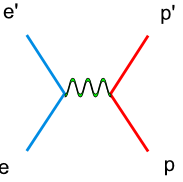
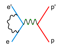
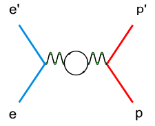
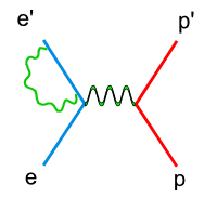
In double spin asymmetry analysis the electron nucleon scattering process is given as an one photon exchange event, so called the Born approximation. In reality, there are multiple photon effects during the experiments. These high order processes, also called radiative effects, can be calculated and used to correct the cross section data.
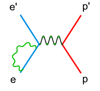
There are two types of radiative corrections, internal and external. Internal radiative corrections describe the contributions which took place during the lepton-hadron interaction. In first order approximation they include vertex photon exchange, self energy and vacuum polarization.<ref name="RadiativeCorrections"> Nucleon Form Factors. In Scholarpedia, from http://www.scholarpedia.org/article/Nucleon_Form_factors#History </ref>
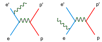
On the other hand, the external radiative corrections account for the Bremsstrahlung by the incoming and scattered electron and by the recoiling target nucleon.
One of the major advantages of the double polarization experiments is the minimum contribution from the radiative corrections. For the ~5.6 GeV incident electron beam data the radiative corrections are less than 5%<ref>http://www.jlab.org/Hall-B/secure/eg1/EG2000/fersch/QUALITY_CHECKS/file_quality/runinfo.txt</ref>. Due to negligible contributions from the radiative corrections they are not included in the double spin asymmetry analysis.
EC CUTS
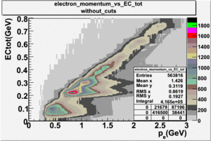
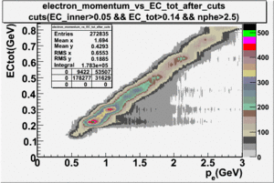
During the EG1b experiment, the electromagnetic calorimeter was used to separate electrons from the pions. The energy deposition into the electromagnetic calorimeter is different for electrons and pions.
Electrons interact with the matter , producing electromagnetic showers and releasing the energy into the matter. The deposited energy into matter is linearly proportional to the momentum of the electrons. On the other hand , pions are minimum ionizing particles(MIP). Traveling through the matter, pions deposit approximately 0.08 GeV energy independent of their momentum.
- Electron Momentum vs EC_total
NPHE CUTS
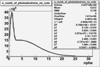
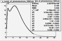
the misidentified electrons were excluded requiring a signal in the threshold CLAS Cherenkov detector. Pion's misidentified as electrons have been shown to produce around ~1.5 photoelectons in the cherenkov detector, as shown below. Geometrical cuts on the location of the particle at the entrance to the cerenkov detector were applied to reduce the pion contamination. The second histogram below shows that after cuts the peak around 1.5 is substantially reduced.
| No cuts | OSI Cuts |
Cherenkov Theory
When the velocity of a charged particle is greater than the local phase velocity of light or when it enters a medium with different optical properties the charged particle will emit photons. The Cherenkov light is emitted under a constant angle - the angle of Cherenkov radiation relative to the particle's direction. It can be shown geometrically that the cosine of the Cherenkov radiation angle is anti-proportional to the velocity of the charged particle
where is the particle's velocity and n - index of refraction of the medium.The charged particle in time t travels distance, while the electromagnetic waves - . For a medium with given index of refraction n there is a threshold velocity , below no radiation can take place. This process may be used to observe the passage of charged particles in a detector which can measure the produced photons.
The number of photons produced per unit path length of a particle with charge ze and per unit energy interval of the photons is proportional to the sine of the Cherenkov angle[1]
after deriving the Taylor expansion of our function and considering only the first two terms, we get
The gas used in the CLAS Cerenkov counter is perfluorobutane with index of refraction equal to 1.00153.
Electrons
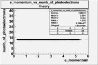
The calculation of the number of photoelectrons emitted by electrons is shown below.
Electron mass , and , because mass of the electron is negligible and also
The Hall B cherenkov detector is m thick radiator. We assume the PMTs used to collect light have a constant quantum efficiency of 8% for photons with wavelength between 300 and 600 nm.
=
- For the number of photoelectrons we have the following
That means the number of photoelectrons should be about 13.
Used file dst27095_05.B00 energy=5.7GeV and torus=2250(B>0). Target NH3
Pions()
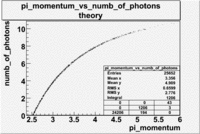
The threshold energy for pions is ~2.5 GeV and for electrons 9 MeV.
- Example for
, momentum and n=1.00153
where
The Hall B cherenkov detector is m thick radiator. We assume the PMTs used to collect light have a constant quantum efficiency of 8% for photons with wavelength between 300 and 600 nm.
=
- For the number of photons we have the following(for pions)
Used file dst27095_05.B00 energy=5.7GeV and torus=2250(B>0). Target NH3
CLAS Cherenkov signal
Electrons
The cherenkov signal measured in CLAS for particles identified as electrons by the tracking algorithm is shown below. There are two distributions present. One distribution is centered around 1.5 PEs and the second distribution is at 8 PEs when two gaussians and a Landau distribution are combined and fit to the spectrum. As we will show below, the first peak is due to the misidentification of a negative pion as an electron.
- PE Fit equation
File:Gaussian fitting function.pdf
C.Lanczos, SIAM Journal of Numerical Analysis B1 (1964), 86.
File:C.Lanczos SIAM Journal of Numerical Analysis B1 1964 86.pdf
normalized fitting functions
Landau and Landaun difference
for me
//__[2] [3] ____________________________________________________________________________
Double_t TMath::Landau(Double_t x, Double_t mpv, Double_t sigma, Bool_t norm)
{
  // The LANDAU function with mpv(most probable value) and sigma.
  // This function has been adapted from the CERNLIB routine G110 denlan.
  // If norm=kTRUE (default is kFALSE) the result is divided by sigma
  static Double_t p1[5] = {0.4259894875,-0.1249762550, 0.03984243700, -0.006298287635,   0.001511162253};
  static Double_t q1[5] = {1.0         ,-0.3388260629, 0.09594393323, -0.01608042283,    0.003778942063};
  static Double_t p2[5] = {0.1788541609, 0.1173957403, 0.01488850518, -0.001394989411,   0.0001283617211};
  static Double_t q2[5] = {1.0         , 0.7428795082, 0.3153932961,   0.06694219548,    0.008790609714};
  static Double_t p3[5] = {0.1788544503, 0.09359161662,0.006325387654, 0.00006611667319,-0.000002031049101};
  static Double_t q3[5] = {1.0         , 0.6097809921, 0.2560616665,   0.04746722384,    0.006957301675};
  static Double_t p4[5] = {0.9874054407, 118.6723273,  849.2794360,   -743.7792444,      427.0262186};
  static Double_t q4[5] = {1.0         , 106.8615961,  337.6496214,    2016.712389,      1597.063511};
  static Double_t p5[5] = {1.003675074,  167.5702434,  4789.711289,    21217.86767,     -22324.94910};
  static Double_t q5[5] = {1.0         , 156.9424537,  3745.310488,    9834.698876,      66924.28357};
  static Double_t p6[5] = {1.000827619,  664.9143136,  62972.92665,    475554.6998,     -5743609.109};
  static Double_t q6[5] = {1.0         , 651.4101098,  56974.73333,    165917.4725,     -2815759.939};
  static Double_t a1[3] = {0.04166666667,-0.01996527778, 0.02709538966};
  static Double_t a2[2] = {-1.845568670,-4.284640743};
  if (sigma <= 0) return 0;
  Double_t v = (x-mpv)/sigma;
  Double_t u, ue, us, den;
  if (v < -5.5) {
     u   = TMath::Exp(v+1.0);
     if (u < 1e-10) return 0.0;
     ue  = TMath::Exp(-1/u);
     us  = TMath::Sqrt(u);
     den = 0.3989422803*(ue/us)*(1+(a1[0]+(a1[1]+a1[2]*u)*u)*u);
  } else if(v < -1) {
     u   = TMath::Exp(-v-1);
     den = TMath::Exp(-u)*TMath::Sqrt(u)*
            (p1[0]+(p1[1]+(p1[2]+(p1[3]+p1[4]*v)*v)*v)*v)/
            (q1[0]+(q1[1]+(q1[2]+(q1[3]+q1[4]*v)*v)*v)*v);
  } else if(v < 1) {
     den = (p2[0]+(p2[1]+(p2[2]+(p2[3]+p2[4]*v)*v)*v)*v)/
           (q2[0]+(q2[1]+(q2[2]+(q2[3]+q2[4]*v)*v)*v)*v);
  } else if(v < 5) {
     den = (p3[0]+(p3[1]+(p3[2]+(p3[3]+p3[4]*v)*v)*v)*v)/
           (q3[0]+(q3[1]+(q3[2]+(q3[3]+q3[4]*v)*v)*v)*v);
  } else if(v < 12) {
     u   = 1/v;
     den = u*u*(p4[0]+(p4[1]+(p4[2]+(p4[3]+p4[4]*u)*u)*u)*u)/
               (q4[0]+(q4[1]+(q4[2]+(q4[3]+q4[4]*u)*u)*u)*u);
  } else if(v < 50) {
     u   = 1/v;
     den = u*u*(p5[0]+(p5[1]+(p5[2]+(p5[3]+p5[4]*u)*u)*u)*u)/
               (q5[0]+(q5[1]+(q5[2]+(q5[3]+q5[4]*u)*u)*u)*u);
  } else if(v < 300) {
     u   = 1/v;
     den = u*u*(p6[0]+(p6[1]+(p6[2]+(p6[3]+p6[4]*u)*u)*u)*u)/
               (q6[0]+(q6[1]+(q6[2]+(q6[3]+q6[4]*u)*u)*u)*u);
  } else {
     u   = 1/(v-v*TMath::Log(v)/(v+1));
     den = u*u*(1+(a2[0]+a2[1]*u)*u);
  }
  if (!norm) return den;
  return den/sigma;
}
Fitting the Histograms
root [13] e_numb_of_photoelectrons->Draw();

root [2] g3= new TF1("g3","gaus(0)+landau(3)+gaus(6)",0,20);
To get fit parameters for g3 we should fit individually each of them(gaus(0),landau(3),gaus(6))
root [3] g3->SetParameters(2.3e3,8,8.1,8.6e+3,8.6e-1,1.6,8.6e+3,8.6e-1,1.6,8.6e3)

root [11] e_numb_of_photoelectrons->Fit("g3","R+");
Notes
<references/>
[Go Back]
