Difference between revisions of "OptiM32 HRRL PositronDesign"
| (4 intermediate revisions by the same user not shown) | |||
| Line 1: | Line 1: | ||
| − | |||
=Software= | =Software= | ||
| Line 11: | Line 10: | ||
http://www.muonsinc.com/tiki-index.php?page=G4beamline | http://www.muonsinc.com/tiki-index.php?page=G4beamline | ||
| + | GEANT4 | ||
| + | |||
| + | http://geant4.cern.ch/ | ||
= Quick Start= | = Quick Start= | ||
| Line 107: | Line 109: | ||
A perl script has been written to convert the above list of beamline elements into a G4beamline input file. | A perl script has been written to convert the above list of beamline elements into a G4beamline input file. | ||
| − | [[ | + | [[optim2g4beam.pl]] |
the syntax is | the syntax is | ||
| Line 278: | Line 280: | ||
[[File:Optim_QS_Step6.png | 200 px]] | [[File:Optim_QS_Step6.png | 200 px]] | ||
| + | |||
| + | click on the "Browse" button in the GUI to load in your file. | ||
| + | |||
| + | :Note; it is probably best to launch the GUI from the same directory which contains all the above *.in files. | ||
== creating virtual detectors== | == creating virtual detectors== | ||
| Line 300: | Line 306: | ||
place Det z=3200 rename=fc | place Det z=3200 rename=fc | ||
</pre> | </pre> | ||
| + | |||
| + | |||
| + | |||
| + | [[Positrons]] | ||
Latest revision as of 16:12, 4 January 2010
Software
Optim32 beamline design software
http://www-bdnew.fnal.gov/pbar/organizationalchart/lebedev/OptiM/optim.htm
G4Beamline
http://www.muonsinc.com/tiki-index.php?page=G4beamline
GEANT4
Quick Start
The instruction below assume you have successfully installed the software above.
Create the *.in files
On the windows machine you can open the file below which represent one design for the HRRL positron source
File:Optim32 HRRL Design Script V1.0.txt
save the above file as HRRL.opt.
The launch the Optim executable by double clicking.
After it is launched click on the "file" menu in the GUI and select the "Open" menu item to choose the file HRRL.opt.
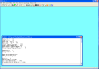
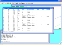
After it is loaded you should see the following below.
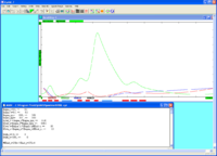
If you click on the icon with the symbols (9th button from the end of the tool bar) you can get a plot of the beam dispersion
This is an interactive display. You can adjust values in the loaded text vile and watch their effect on the dispersion. Notice the colored rectangles at the colored rectangles at the bottom of the beta curve sub window. Starting from the left bottom there are 3 read rectangles , a blue rectangle, then 3 red rectangles, a blue rectangle, and finally 3 more red rectangles. The red rectangles are the quadrupoles in the beam line and the blue rectangles are the dipoles. If you click on them their element name will appear in the upper right corner of the dispersion sub window.
If you scroll down the HRRL.opt input file to line which says
begin list
you will se a list of all the elements, the B-field values, their lengths, etc...
If you scroll down to the first quad
q0 L[cm]=13 G[kG/cm]=0.0438324 Tilt[deg]=0
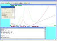
you can move the curser the the B-field value "G[kG/cm]=0.0438324" and increment it while watch the effect on the dispersion plot. You increments it hitting the left and right arrow keys while holding down the "Crtl" key. The value of the increment step is controlled by through the parameters available in the dialog box you get when you select "Steps" from the "Edit" menu.
The above says the quadrupole B-field step size is set to 0.005.
Let's assume you have finished a design and now you would like to simulate the beam line using G4beamline.
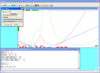
Create a text file by selecting "Lattice" from the "View" menu (Alt-L is the shortcut key) and click OK when the dialog box appears below.
Clicking "OK" in the dialog box will cause a text window to open up which looks like the image below.
Save the list of elements to a text file. The text window contains other text you don't need for G4bemline. The following is the text file which was written for this example
N 	Name 	S[cm] 	L[cm] 	B[kG] 	G[kG/cm]   S[kG/cm/cm] 	Tilt[deg] 	Tilt_out 	BendAng[deg]
1 	oD0 	4.03293 	4.03293
2 	q0 	17.0329 	13 	0 	0.0338324 	0 	0
3 	oD1 	20.5462 	3.51326
4 	q1 	33.5462 	13 	0 	-0.0651436 	0 	0
5 	oD2 	39.5285 	5.9823
6 	q2 	52.5285 	13 	0 	0.0449155 	0 	0
7 	oD3 	62.18 	9.65149
8 	gC1 	62.18 	0 	0  Angle[deg]=0  Eff.Length[cm]=0  Tilt[deg]=0
9 	bC1 	92.18 	30 	-0.315179 	0 	0 	0 	0 	-54.1377
10 	GC1 	92.18 	0 	0  Angle[deg]=0  Eff.Length[cm]=0  Tilt[deg]=0
11 	oD7 	108.98 	16.8
12 	q6 	121.98 	13 	0 	-0.0190153 	0 	0
13 	oD8 	132.68 	10.7
14 	q7 	145.68 	13 	0 	0.0365559 	0 	0
15 	oD9 	158.13 	12.45
16 	q8 	171.13 	13 	0 	-0.0231326 	0 	0
17 	oD10 	182.03 	10.9
18 	gC2 	182.03 	0 	0  Angle[deg]=0  Eff.Length[cm]=0  Tilt[deg]=0
19 	bC2 	212.03 	30 	-0.285179 	0 	0 	0 	0 	-48.9847
20 	GC2 	212.03 	0 	0  Angle[deg]=0  Eff.Length[cm]=0  Tilt[deg]=0
21 	oD11 	242.03 	30
22 	q9 	262.03 	20 	0 	0.0119605 	0 	0
23 	oD12 	266.541 	4.51061
24 	q10 	286.541 	20 	0 	-0.00837701 	0 	0
25 	oD13 	292.532 	5.99133
26 	q11 	312.532 	20 	0 	0.0031277 	0 	0
27 	oD14 	513.032 	200.5
- Save the above file under the file HRRL.txt or any simular name
Converting text file for G4beamline
A perl script has been written to convert the above list of beamline elements into a G4beamline input file.
the syntax is
perl optim2g4beam.pl HRRL.txt
The perl script write the file z_positions.in based on the contents of the HRRL.txt file.
Below is the resulting z_positions.in file
place QType13 gradient=0.518324 z=105.33 rename=q0
place QType13 gradient=-0.631436 z=270.46 rename=q1
place QType13 gradient=0.239155 z=460.29 rename=q2
tune bC1 z0=471.16 z1=971.16 initial=-0.03151790 step=0.00001 expr=atan(Px1/Pz1) tolerance=0.0000001
place SECT_BEND2 By=bC1 z=-0.032 rename=571.164
cornerarc C1 z=571.164 centerRadius=381.971943 angle=45.000000
place QType13 gradient=-0.190153 z=1104.16 rename=q6
place QType13 gradient=0.415559 z=1341.16 rename=q7
place QType13 gradient=-0.228326 z=1595.66 rename=q8
tune bC1 z0=1619.03 z1=2119.03 initial=-0.03151790 step=0.00001 expr=atan(Px1/Pz1) tolerance=0.0000001
place SECT_BEND2 By=bC1 z=-0.032 rename=1719.03
cornerarc C1 z=1719.030 centerRadius=381.971943 angle=45.000000
place QType20 gradient=-0.010395 z=2419.03 rename=q9
place QType20 gradient=0.056230 z=2664.13 rename=q10
place QType20 gradient=-0.008723 z=2924.05 rename=q11
Currently there is a bug in the perl script such that the 90 degree bending magnet "bC1" has its name repeated and the z position is a negative number because the actual z position is listed after the "rename=" field
so change line 10 and 11 from
tune bC1 z0=471.16 z1=971.16 initial=-0.03151790 step=0.00001 expr=atan(Px1/Pz1) tolerance=0.0000001
place SECT_BEND2 By=bC1 z=-0.032 rename=571.164
to
tune bC1 z0=471.16 z1=971.16 initial=-0.03151790 step=0.001 expr=atan(Px1/Pz1) tolerance=0.0001
place SECT_BEND2 By=bC1 z=571.164 rename=571.164
and line 15 and 16 from
 tune bC1 z0=1619.03 z1=2119.03 initial=-0.03151790 step=0.00001 expr=atan(Px1/Pz1) tolerance=0.0000001
place SECT_BEND2 By=bC1 z=-0.032 rename=1719.03
to
tune bC2 z0=1619.03 z1=2119.03 initial=-0.03151790 step=0.001 expr=atan(Px1/Pz1) tolerance=0.0001
place SECT_BEND2 By=bC2 z=1719.03 rename=1719.03
the correct file should look like
place QType13 gradient=0.518324 z=105.33 rename=q0
place QType13 gradient=-0.631436 z=270.46 rename=q1
place QType13 gradient=0.239155 z=460.29 rename=q2
tune bC1 z0=471.16 z1=971.16 initial=-0.03151790 step=0.001 expr=atan(Px1/Pz1) tolerance=0.0001
place SECT_BEND2 By=bC1 z=571.164 rename=571.164
cornerarc C1 z=571.164 centerRadius=381.971943 angle=45.000000
place QType13 gradient=-0.190153 z=1104.16 rename=q6
place QType13 gradient=0.415559 z=1341.16 rename=q7
place QType13 gradient=-0.228326 z=1595.66 rename=q8
tune bC2 z0=1619.03 z1=2119.03 initial=-0.03151790 step=0.001 expr=atan(Px1/Pz1) tolerance=0.0001
place SECT_BEND2 By=bC2 z=1719.03 rename=1719.03
cornerarc C1 z=1719.030 centerRadius=381.971943 angle=45.000000
place QType20 gradient=-0.010395 z=2419.03 rename=q9
place QType20 gradient=0.056230 z=2664.13 rename=q10
place QType20 gradient=-0.008723 z=2924.05 rename=q11
Running G4beamline
To run G4 beamline you can use the following skeleton file which includes several other input files. In this example the beam energy is 3 MeV.
physics QGSP_BIC

param -unset P=3

include parameters_3MeV.in

reference referenceMomentum=$P particle=e+ beamZ=0.0

trackcuts keep=gamma,e-,e+ kineticEnergyCut=0.01 killSecondaries=0

beam gaussian particle=e+ nEvents=600 beamZ=0.0\
sigmaX=1. sigmaY=1. sigmaXp=0.01 sigmaYp=0.01\
meanMomentum=$P sigmaP=0.3 meanT=0.0 sigmaT=0.020

include z_positions.in
notice there are 2 other input files called "parameters_3Mev.in" and "z_positions.in"
The parameters file looks like:
#Length of Detectors and Particle Filters #
param -unset PI=3.14159265
param -unset DL=0.0001
param -unset L_QType13=130.0
param -unset L_QType20=200.0
param -unset B1=0
param -unset bend_ang1=45
param -unset bend_ang2=45
param -unset L_of_S1=300.0
param -unset deg2rad=$PI/180.0
# Bend field in Tesla
#Does not work param -unset B_bend=(1/100)*(299.8)*$P*($deg2rad*$bend_ang1)/($L_of_S1)
param -unset B_bend=1
#Bending radius in mm
param -unset rho1=$L_of_S1/($deg2rad*abs($bend_ang1))
param -unset rho2=$rho1

#param -unset rho1=$L_of_S1/($bend_ang1*$PI/180)
#param -unset rho2=(2*$L_of_S1)/($bend_ang2*$PI/180)
param -unset kill_all=1
param -unset Dip_Gap_Aper=50.0
param -unset pipe_1_Radi=10.5
param -unset Q13_Radi=60.0
param -unset Corr_W=195
param -unset Corr_L=50.0
param -unset L_RF_Cell=100.0
param -unset L_RF_Cell_Ef=70.0
param -unset collim_in=2.5

trackcuts keep=gamma,e-,e+ kineticEnergyCut=0.01 killSecondaries=0

genericbend Corrector fieldWidth=$Corr_W fieldHeight=$Corr_W fieldLength=$Corr_L\
ironWidth=$Corr_W*1.21 ironHeight=$Corr_W*1.21 ironLength=$Corr_L\
By=$B1 fieldMaterial=Vacuum ironMaterial=Air\
ironColor=0,1,1 kill=$kill_all fringe=0

idealsectorbend SECT_BEND1 angle=$bend_ang1 fieldCenterRadius=$rho1\
fieldInnerRadius=($rho1*0.92) fieldOuterRadius=($rho1*1.2) fieldHeight=$Dip_Gap_Aper\
ironInnerRadius=($rho1*0.89) ironOuterRadius=($rho1*1.4) ironHeight=(1.5*$Dip_Gap_Aper)\
By=$B1 ironColor=1,0,0 kill=$kill_all

idealsectorbend SECT_BEND2 angle=$bend_ang2 fieldCenterRadius=$rho2\
fieldInnerRadius=($rho2*0.92) fieldOuterRadius=($rho2*1.2) fieldHeight=$Dip_Gap_Aper\
ironInnerRadius=($rho2*0.89) ironOuterRadius=($rho2*1.4) ironHeight=(1.5*$Dip_Gap_Aper)\
By=$B1 ironColor=1,0,0 kill=$kill_all
#genericquad QType15 apertureRadius=$Q15_Radi ironRadius=(1.75*$Q15_Radi) ironColor=1,1,0\
#kill=$kill_all fringe=0 fieldLength=$L_QType15 ironLength=$L_QType15
genericquad QType13 apertureRadius=$Q13_Radi ironRadius=(1.75*$Q13_Radi) ironColor=1,1,0\
kill=$kill_all fringe=0 fieldLength=$L_QType13 ironLength=$L_QType13

genericquad QType20 apertureRadius=$Q13_Radi ironRadius=(1.75*$Q13_Radi) ironColor=1,1,0\
kill=$kill_all fringe=0 fieldLength=$L_QType20 ironLength=$L_QType20


tubs pipe_1 innerRadius=($pipe_1_Radi-0.5) outerRadius=$pipe_1_Radi length=1 material=Fe color=0.5,0.5,1 kill=$kill_all

tubs Collimator innerRadius=$collim_in outerRadius=(50*$collim_in) length=0.1 material=Fe color=0.5,0.5,1 kill=1
tubs Collimator1 innerRadius=6 outerRadius=(5000) length=5 material=Fe color=0.5,0.5,1 kill=1

particlefilter PF radius=100 length=$DL color=1,1,0.5 kill=e-,gamma keep=e+ require=1

#virtualdetector Det radius=($pipe_1_Radi-0.5) length=$DL color=1,0.1,0.7 format=BLTrackfile
#virtualdetector Det radius=20.5 length=0.00001 color=1,0.1,0.7 format=BLTrackfile
virtualdetector Det radius=100.5 length=0.00001 color=1,0.1,0.7 format=root
The "z_positons.in" file is given in the previous section. Notice the last line above has defined a virtual detector. We will use later in a section below.
- You can now run the G4beamline GUI, if it is in your path, by typing "g4blgui"
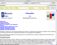
Below is a screen shot of the GUI
click on the "Browse" button in the GUI to load in your file.
- Note; it is probably best to launch the GUI from the same directory which contains all the above *.in files.
creating virtual detectors
Virtual detector may be created to intercept the particles traveling down the beam pipe to record their momentum and position at specified locations along the beam line.
place QType13 gradient=0.518324 z=105.33 rename=q0
place QType13 gradient=-0.631436 z=270.46 rename=q1
place QType13 gradient=0.239155 z=460.29 rename=q2
tune bC1 z0=471.16 z1=971.16 initial=-0.03151790 step=0.001 expr=atan(Px1/Pz1) tolerance=0.0001
place SECT_BEND2 By=bC1 z=571.164 rename=571.164
cornerarc C1 z=571.164 centerRadius=381.971943 angle=45.000000
place QType13 gradient=-0.190153 z=1104.16 rename=q6
place QType13 gradient=0.415559 z=1341.16 rename=q7
place QType13 gradient=-0.228326 z=1595.66 rename=q8
tune bC2 z0=1619.03 z1=2119.03 initial=-0.03151790 step=0.001 expr=atan(Px1/Pz1) tolerance=0.0001
place SECT_BEND2 By=bC2 z=1719.03 rename=1719.03
cornerarc C1 z=1719.030 centerRadius=381.971943 angle=45.000000
place QType20 gradient=-0.010395 z=2419.03 rename=q9
place QType20 gradient=0.056230 z=2664.13 rename=q10
place QType20 gradient=-0.008723 z=2924.05 rename=q11
place Det z=3200 rename=fc
