Difference between revisions of "Analysis"
| Line 1,102: | Line 1,102: | ||
<math>\left ( \begin{matrix} p_{\pi x}^{LAB{\prime}} \\ p_{\pi y}^{LAB{\prime}} \\p_{\pi z}^{LAB{\prime}} \end{matrix} \right )= \left [ \begin{matrix} cos {\theta}_x & 0 & -sin {\theta_x} \\ 0 & 1 &0 \\ sin {\theta_x} &0 & cos {\theta_x} \end{matrix} \right ] \left [ \begin{matrix} cos {\phi} & sin {\phi} & 0 \\ -sin {\phi} & cos {\phi} &0 \\ 0 &0 & 1 \end{matrix} \right ] \left ( \begin{matrix} p_{\pi x}^{LAB} \\p_{\pi y}^{LAB} \\ p_{\pi z}^{LAB} \end{matrix} \right ) = </math> <br> | <math>\left ( \begin{matrix} p_{\pi x}^{LAB{\prime}} \\ p_{\pi y}^{LAB{\prime}} \\p_{\pi z}^{LAB{\prime}} \end{matrix} \right )= \left [ \begin{matrix} cos {\theta}_x & 0 & -sin {\theta_x} \\ 0 & 1 &0 \\ sin {\theta_x} &0 & cos {\theta_x} \end{matrix} \right ] \left [ \begin{matrix} cos {\phi} & sin {\phi} & 0 \\ -sin {\phi} & cos {\phi} &0 \\ 0 &0 & 1 \end{matrix} \right ] \left ( \begin{matrix} p_{\pi x}^{LAB} \\p_{\pi y}^{LAB} \\ p_{\pi z}^{LAB} \end{matrix} \right ) = </math> <br> | ||
| − | <math>= \left ( \begin{matrix} cos {\theta}_x | + | <math>= \left ( \begin{matrix} cos {\theta}_x (cos {\phi} p_{\pi x}^{LAB} + sin {\phi} p_{\pi y}^{LAB}) - sin {\theta}_x p_{\pi z}^{LAB} \\ -sin {\phi} p_{\pi x}^{LAB} + cos {\phi} p_{\pi y}^{LAB} \\ sin {\theta}_x (cos {\phi} p_{\pi x}^{LAB} + sin {\phi} p_{\pi y}^{LAB}) + cos {\theta}_x p_{\pi z}^{LAB} \end{matrix} \right ) </math><br> |
now rotate about <math>\phi</math> angle | now rotate about <math>\phi</math> angle | ||
Revision as of 23:02, 19 February 2008
EG1 run database
run summary
polarization info
Particle Identification
Cherenkov
Cherenkov Theory
When the velocity of a charged particle is greater than the local phase velocity of light or when it enters a medium with different optical properties the charged particle will emit photons. The Cherenkov light is emitted under a constant angle - the angle of Cherenkov radiation relative to the particle's direction. It can be shown geometrically that the cosine of the Cherenkov radiation angle is anti-proportional to the velocity of the charged particle
where is the particle's velocity and n - index of refraction of the medium.The charged particle in time t travels distance, while the electromagnetic waves - . For a medium with given index of refraction n there is a threshold velocity , below no radiation can take place. This process may be used to observe the passage of charged particles in a detector which can measure the produced photons.
The number of photons produced per unit path length of a particle with charge ze and per unit energy interval of the photons is proportional to the sine of the Cherenkov angle[1]
after deriving the Taylor expansion of our function and considering only the first two terms, we get
The gas used in the CLAS Cerenkov counter is perfluorobutane with index of refraction equal to 1.00153.
Electrons
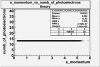
The calculation of the number of photoelectrons emitted by electrons is shown below.
Electron mass , and , because mass of the electron is negligible and also
The Hall B cherenkov detector is m thick radiator. We assume the PMTs used to collect light have a constant quantum efficiency of 8% for photons with wavelength between 300 and 600 nm.
=
- For the number of photoelectrons we have the following
That means the number of photoelectrons should be about 13.
Used file dst27095_05.B00 energy=5.7GeV and torus=2250(B>0). Target NH3
Pions()
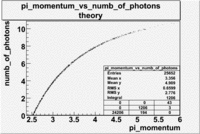
The threshold energy for pions is ~2.5 GeV and for electrons 9 MeV.
- Example for
, momentum and n=1.00153
where
The Hall B cherenkov detector is m thick radiator. We assume the PMTs used to collect light have a constant quantum efficiency of 8% for photons with wavelength between 300 and 600 nm.
=
- For the number of photons we have the following(for pions)
Used file dst27095_05.B00 energy=5.7GeV and torus=2250(B>0). Target NH3
CLAS Cherenkov signal
Electrons
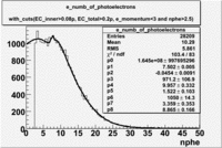
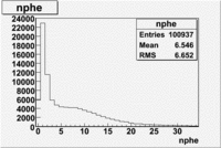
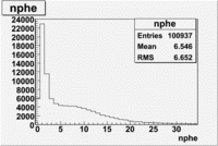
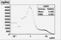
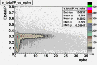
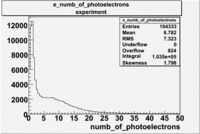
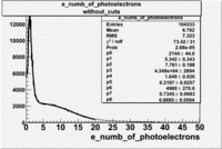
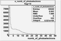
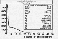
The cherenkov signal measured in CLAS for particles identified as electrons by the tracking algorithm is shown below. There are two distributions present. One distribution is centered around 1.5 PEs and the second distribution is at 8 PEs when two gaussians and a Landau distribution are combined and fit to the spectrum. As we will show below, the first peak is due to the misidentification of a negative pion as an electron.
- PE Fit equation
File:Gaussian fitting function.pdf
C.Lanczos, SIAM Journal of Numerical Analysis B1 (1964), 86.
File:C.Lanczos SIAM Journal of Numerical Analysis B1 1964 86.pdf
//__[2] [3] ____________________________________________________________________________
Double_t TMath::Landau(Double_t x, Double_t mpv, Double_t sigma, Bool_t norm)
{
  // The LANDAU function with mpv(most probable value) and sigma.
  // This function has been adapted from the CERNLIB routine G110 denlan.
  // If norm=kTRUE (default is kFALSE) the result is divided by sigma
  static Double_t p1[5] = {0.4259894875,-0.1249762550, 0.03984243700, -0.006298287635,   0.001511162253};
  static Double_t q1[5] = {1.0         ,-0.3388260629, 0.09594393323, -0.01608042283,    0.003778942063};
  static Double_t p2[5] = {0.1788541609, 0.1173957403, 0.01488850518, -0.001394989411,   0.0001283617211};
  static Double_t q2[5] = {1.0         , 0.7428795082, 0.3153932961,   0.06694219548,    0.008790609714};
  static Double_t p3[5] = {0.1788544503, 0.09359161662,0.006325387654, 0.00006611667319,-0.000002031049101};
  static Double_t q3[5] = {1.0         , 0.6097809921, 0.2560616665,   0.04746722384,    0.006957301675};
  static Double_t p4[5] = {0.9874054407, 118.6723273,  849.2794360,   -743.7792444,      427.0262186};
  static Double_t q4[5] = {1.0         , 106.8615961,  337.6496214,    2016.712389,      1597.063511};
  static Double_t p5[5] = {1.003675074,  167.5702434,  4789.711289,    21217.86767,     -22324.94910};
  static Double_t q5[5] = {1.0         , 156.9424537,  3745.310488,    9834.698876,      66924.28357};
  static Double_t p6[5] = {1.000827619,  664.9143136,  62972.92665,    475554.6998,     -5743609.109};
  static Double_t q6[5] = {1.0         , 651.4101098,  56974.73333,    165917.4725,     -2815759.939};
  static Double_t a1[3] = {0.04166666667,-0.01996527778, 0.02709538966};
  static Double_t a2[2] = {-1.845568670,-4.284640743};
  if (sigma <= 0) return 0;
  Double_t v = (x-mpv)/sigma;
  Double_t u, ue, us, den;
  if (v < -5.5) {
     u   = TMath::Exp(v+1.0);
     if (u < 1e-10) return 0.0;
     ue  = TMath::Exp(-1/u);
     us  = TMath::Sqrt(u);
     den = 0.3989422803*(ue/us)*(1+(a1[0]+(a1[1]+a1[2]*u)*u)*u);
  } else if(v < -1) {
     u   = TMath::Exp(-v-1);
     den = TMath::Exp(-u)*TMath::Sqrt(u)*
            (p1[0]+(p1[1]+(p1[2]+(p1[3]+p1[4]*v)*v)*v)*v)/
            (q1[0]+(q1[1]+(q1[2]+(q1[3]+q1[4]*v)*v)*v)*v);
  } else if(v < 1) {
     den = (p2[0]+(p2[1]+(p2[2]+(p2[3]+p2[4]*v)*v)*v)*v)/
           (q2[0]+(q2[1]+(q2[2]+(q2[3]+q2[4]*v)*v)*v)*v);
  } else if(v < 5) {
     den = (p3[0]+(p3[1]+(p3[2]+(p3[3]+p3[4]*v)*v)*v)*v)/
           (q3[0]+(q3[1]+(q3[2]+(q3[3]+q3[4]*v)*v)*v)*v);
  } else if(v < 12) {
     u   = 1/v;
     den = u*u*(p4[0]+(p4[1]+(p4[2]+(p4[3]+p4[4]*u)*u)*u)*u)/
               (q4[0]+(q4[1]+(q4[2]+(q4[3]+q4[4]*u)*u)*u)*u);
  } else if(v < 50) {
     u   = 1/v;
     den = u*u*(p5[0]+(p5[1]+(p5[2]+(p5[3]+p5[4]*u)*u)*u)*u)/
               (q5[0]+(q5[1]+(q5[2]+(q5[3]+q5[4]*u)*u)*u)*u);
  } else if(v < 300) {
     u   = 1/v;
     den = u*u*(p6[0]+(p6[1]+(p6[2]+(p6[3]+p6[4]*u)*u)*u)*u)/
               (q6[0]+(q6[1]+(q6[2]+(q6[3]+q6[4]*u)*u)*u)*u);
  } else {
     u   = 1/(v-v*TMath::Log(v)/(v+1));
     den = u*u*(1+(a2[0]+a2[1]*u)*u);
  }
  if (!norm) return den;
  return den/sigma;
}
Below is the source code from root to generate a random number from a Landau distribution
//______________________________________________________________________________
Double_t TRandom::Landau(Double_t mpv, Double_t sigma)
{
//  Generate a random number following a Landau distribution
//  with mpv(most probable value) and sigma
//  Converted by Rene Brun from CERNLIB routine ranlan(G110)
  static Double_t f[982] = {
      0       , 0       , 0       ,0        ,0        ,-2.244733,
     -2.204365,-2.168163,-2.135219,-2.104898,-2.076740,-2.050397,
     -2.025605,-2.002150,-1.979866,-1.958612,-1.938275,-1.918760,
     -1.899984,-1.881879,-1.864385,-1.847451,-1.831030,-1.815083,
     -1.799574,-1.784473,-1.769751,-1.755383,-1.741346,-1.727620,
     -1.714187,-1.701029,-1.688130,-1.675477,-1.663057,-1.650858,
     -1.638868,-1.627078,-1.615477,-1.604058,-1.592811,-1.581729,
     -1.570806,-1.560034,-1.549407,-1.538919,-1.528565,-1.518339,
     -1.508237,-1.498254,-1.488386,-1.478628,-1.468976,-1.459428,
     -1.449979,-1.440626,-1.431365,-1.422195,-1.413111,-1.404112,
     -1.395194,-1.386356,-1.377594,-1.368906,-1.360291,-1.351746,
     -1.343269,-1.334859,-1.326512,-1.318229,-1.310006,-1.301843,
     -1.293737,-1.285688,-1.277693,-1.269752,-1.261863,-1.254024,
     -1.246235,-1.238494,-1.230800,-1.223153,-1.215550,-1.207990,
     -1.200474,-1.192999,-1.185566,-1.178172,-1.170817,-1.163500,
     -1.156220,-1.148977,-1.141770,-1.134598,-1.127459,-1.120354,
     -1.113282,-1.106242,-1.099233,-1.092255,
     -1.085306,-1.078388,-1.071498,-1.064636,-1.057802,-1.050996,
     -1.044215,-1.037461,-1.030733,-1.024029,-1.017350,-1.010695,
     -1.004064, -.997456, -.990871, -.984308, -.977767, -.971247,
      -.964749, -.958271, -.951813, -.945375, -.938957, -.932558,
      -.926178, -.919816, -.913472, -.907146, -.900838, -.894547,
      -.888272, -.882014, -.875773, -.869547, -.863337, -.857142,
      -.850963, -.844798, -.838648, -.832512, -.826390, -.820282,
      -.814187, -.808106, -.802038, -.795982, -.789940, -.783909,
      -.777891, -.771884, -.765889, -.759906, -.753934, -.747973,
      -.742023, -.736084, -.730155, -.724237, -.718328, -.712429,
      -.706541, -.700661, -.694791, -.688931, -.683079, -.677236,
      -.671402, -.665576, -.659759, -.653950, -.648149, -.642356,
      -.636570, -.630793, -.625022, -.619259, -.613503, -.607754,
      -.602012, -.596276, -.590548, -.584825, -.579109, -.573399,
      -.567695, -.561997, -.556305, -.550618, -.544937, -.539262,
      -.533592, -.527926, -.522266, -.516611, -.510961, -.505315,
      -.499674, -.494037, -.488405, -.482777,
      -.477153, -.471533, -.465917, -.460305, -.454697, -.449092,
      -.443491, -.437893, -.432299, -.426707, -.421119, -.415534,
      -.409951, -.404372, -.398795, -.393221, -.387649, -.382080,
      -.376513, -.370949, -.365387, -.359826, -.354268, -.348712,
      -.343157, -.337604, -.332053, -.326503, -.320955, -.315408,
      -.309863, -.304318, -.298775, -.293233, -.287692, -.282152,
      -.276613, -.271074, -.265536, -.259999, -.254462, -.248926,
      -.243389, -.237854, -.232318, -.226783, -.221247, -.215712,
      -.210176, -.204641, -.199105, -.193568, -.188032, -.182495,
      -.176957, -.171419, -.165880, -.160341, -.154800, -.149259,
      -.143717, -.138173, -.132629, -.127083, -.121537, -.115989,
      -.110439, -.104889, -.099336, -.093782, -.088227, -.082670,
      -.077111, -.071550, -.065987, -.060423, -.054856, -.049288,
      -.043717, -.038144, -.032569, -.026991, -.021411, -.015828,
      -.010243, -.004656,  .000934,  .006527,  .012123,  .017722,
       .023323,  .028928,  .034535,  .040146,  .045759,  .051376,
       .056997,  .062620,  .068247,  .073877,
       .079511,  .085149,  .090790,  .096435,  .102083,  .107736,
       .113392,  .119052,  .124716,  .130385,  .136057,  .141734,
       .147414,  .153100,  .158789,  .164483,  .170181,  .175884,
       .181592,  .187304,  .193021,  .198743,  .204469,  .210201,
       .215937,  .221678,  .227425,  .233177,  .238933,  .244696,
       .250463,  .256236,  .262014,  .267798,  .273587,  .279382,
       .285183,  .290989,  .296801,  .302619,  .308443,  .314273,
       .320109,  .325951,  .331799,  .337654,  .343515,  .349382,
       .355255,  .361135,  .367022,  .372915,  .378815,  .384721,
       .390634,  .396554,  .402481,  .408415,  .414356,  .420304,
       .426260,  .432222,  .438192,  .444169,  .450153,  .456145,
       .462144,  .468151,  .474166,  .480188,  .486218,  .492256,
       .498302,  .504356,  .510418,  .516488,  .522566,  .528653,
       .534747,  .540850,  .546962,  .553082,  .559210,  .565347,
       .571493,  .577648,  .583811,  .589983,  .596164,  .602355,
       .608554,  .614762,  .620980,  .627207,  .633444,  .639689,
       .645945,  .652210,  .658484,  .664768,
       .671062,  .677366,  .683680,  .690004,  .696338,  .702682,
       .709036,  .715400,  .721775,  .728160,  .734556,  .740963,
       .747379,  .753807,  .760246,  .766695,  .773155,  .779627,
       .786109,  .792603,  .799107,  .805624,  .812151,  .818690,
       .825241,  .831803,  .838377,  .844962,  .851560,  .858170,
       .864791,  .871425,  .878071,  .884729,  .891399,  .898082,
       .904778,  .911486,  .918206,  .924940,  .931686,  .938446,
       .945218,  .952003,  .958802,  .965614,  .972439,  .979278,
       .986130,  .992996,  .999875, 1.006769, 1.013676, 1.020597,
      1.027533, 1.034482, 1.041446, 1.048424, 1.055417, 1.062424,
      1.069446, 1.076482, 1.083534, 1.090600, 1.097681, 1.104778,
      1.111889, 1.119016, 1.126159, 1.133316, 1.140490, 1.147679,
      1.154884, 1.162105, 1.169342, 1.176595, 1.183864, 1.191149,
      1.198451, 1.205770, 1.213105, 1.220457, 1.227826, 1.235211,
      1.242614, 1.250034, 1.257471, 1.264926, 1.272398, 1.279888,
      1.287395, 1.294921, 1.302464, 1.310026, 1.317605, 1.325203,
      1.332819, 1.340454, 1.348108, 1.355780,
      1.363472, 1.371182, 1.378912, 1.386660, 1.394429, 1.402216,
      1.410024, 1.417851, 1.425698, 1.433565, 1.441453, 1.449360,
      1.457288, 1.465237, 1.473206, 1.481196, 1.489208, 1.497240,
      1.505293, 1.513368, 1.521465, 1.529583, 1.537723, 1.545885,
      1.554068, 1.562275, 1.570503, 1.578754, 1.587028, 1.595325,
      1.603644, 1.611987, 1.620353, 1.628743, 1.637156, 1.645593,
      1.654053, 1.662538, 1.671047, 1.679581, 1.688139, 1.696721,
      1.705329, 1.713961, 1.722619, 1.731303, 1.740011, 1.748746,
      1.757506, 1.766293, 1.775106, 1.783945, 1.792810, 1.801703,
      1.810623, 1.819569, 1.828543, 1.837545, 1.846574, 1.855631,
      1.864717, 1.873830, 1.882972, 1.892143, 1.901343, 1.910572,
      1.919830, 1.929117, 1.938434, 1.947781, 1.957158, 1.966566,
      1.976004, 1.985473, 1.994972, 2.004503, 2.014065, 2.023659,
      2.033285, 2.042943, 2.052633, 2.062355, 2.072110, 2.081899,
      2.091720, 2.101575, 2.111464, 2.121386, 2.131343, 2.141334,
      2.151360, 2.161421, 2.171517, 2.181648, 2.191815, 2.202018,
      2.212257, 2.222533, 2.232845, 2.243195,
      2.253582, 2.264006, 2.274468, 2.284968, 2.295507, 2.306084,
      2.316701, 2.327356, 2.338051, 2.348786, 2.359562, 2.370377,
      2.381234, 2.392131, 2.403070, 2.414051, 2.425073, 2.436138,
      2.447246, 2.458397, 2.469591, 2.480828, 2.492110, 2.503436,
      2.514807, 2.526222, 2.537684, 2.549190, 2.560743, 2.572343,
      2.583989, 2.595682, 2.607423, 2.619212, 2.631050, 2.642936,
      2.654871, 2.666855, 2.678890, 2.690975, 2.703110, 2.715297,
      2.727535, 2.739825, 2.752168, 2.764563, 2.777012, 2.789514,
      2.802070, 2.814681, 2.827347, 2.840069, 2.852846, 2.865680,
      2.878570, 2.891518, 2.904524, 2.917588, 2.930712, 2.943894,
      2.957136, 2.970439, 2.983802, 2.997227, 3.010714, 3.024263,
      3.037875, 3.051551, 3.065290, 3.079095, 3.092965, 3.106900,
      3.120902, 3.134971, 3.149107, 3.163312, 3.177585, 3.191928,
      3.206340, 3.220824, 3.235378, 3.250005, 3.264704, 3.279477,
      3.294323, 3.309244, 3.324240, 3.339312, 3.354461, 3.369687,
      3.384992, 3.400375, 3.415838, 3.431381, 3.447005, 3.462711,
      3.478500, 3.494372, 3.510328, 3.526370,
      3.542497, 3.558711, 3.575012, 3.591402, 3.607881, 3.624450,
      3.641111, 3.657863, 3.674708, 3.691646, 3.708680, 3.725809,
      3.743034, 3.760357, 3.777779, 3.795300, 3.812921, 3.830645,
      3.848470, 3.866400, 3.884434, 3.902574, 3.920821, 3.939176,
      3.957640, 3.976215, 3.994901, 4.013699, 4.032612, 4.051639,
      4.070783, 4.090045, 4.109425, 4.128925, 4.148547, 4.168292,
      4.188160, 4.208154, 4.228275, 4.248524, 4.268903, 4.289413,
      4.310056, 4.330832, 4.351745, 4.372794, 4.393982, 4.415310,
      4.436781, 4.458395, 4.480154, 4.502060, 4.524114, 4.546319,
      4.568676, 4.591187, 4.613854, 4.636678, 4.659662, 4.682807,
      4.706116, 4.729590, 4.753231, 4.777041, 4.801024, 4.825179,
      4.849511, 4.874020, 4.898710, 4.923582, 4.948639, 4.973883,
      4.999316, 5.024942, 5.050761, 5.076778, 5.102993, 5.129411,
      5.156034, 5.182864, 5.209903, 5.237156, 5.264625, 5.292312,
      5.320220, 5.348354, 5.376714, 5.405306, 5.434131, 5.463193,
      5.492496, 5.522042, 5.551836, 5.581880, 5.612178, 5.642734,
      5.673552, 5.704634, 5.735986, 5.767610,
      5.799512, 5.831694, 5.864161, 5.896918, 5.929968, 5.963316,
      5.996967, 6.030925, 6.065194, 6.099780, 6.134687, 6.169921,
      6.205486, 6.241387, 6.277630, 6.314220, 6.351163, 6.388465,
      6.426130, 6.464166, 6.502578, 6.541371, 6.580553, 6.620130,
      6.660109, 6.700495, 6.741297, 6.782520, 6.824173, 6.866262,
      6.908795, 6.951780, 6.995225, 7.039137, 7.083525, 7.128398,
      7.173764, 7.219632, 7.266011, 7.312910, 7.360339, 7.408308,
      7.456827, 7.505905, 7.555554, 7.605785, 7.656608, 7.708035,
      7.760077, 7.812747, 7.866057, 7.920019, 7.974647, 8.029953,
      8.085952, 8.142657, 8.200083, 8.258245, 8.317158, 8.376837,
      8.437300, 8.498562, 8.560641, 8.623554, 8.687319, 8.751955,
      8.817481, 8.883916, 8.951282, 9.019600, 9.088889, 9.159174,
      9.230477, 9.302822, 9.376233, 9.450735, 9.526355, 9.603118,
      9.681054, 9.760191, 9.840558, 9.922186,10.005107,10.089353,
     10.174959,10.261958,10.350389,10.440287,10.531693,10.624646,
     10.719188,10.815362,10.913214,11.012789,11.114137,11.217307,
     11.322352,11.429325,11.538283,11.649285,
     11.762390,11.877664,11.995170,12.114979,12.237161,12.361791,
     12.488946,12.618708,12.751161,12.886394,13.024498,13.165570,
     13.309711,13.457026,13.607625,13.761625,13.919145,14.080314,
     14.245263,14.414134,14.587072,14.764233,14.945778,15.131877,
     15.322712,15.518470,15.719353,15.925570,16.137345,16.354912,
     16.578520,16.808433,17.044929,17.288305,17.538873,17.796967,
     18.062943,18.337176,18.620068,18.912049,19.213574,19.525133,
     19.847249,20.180480,20.525429,20.882738,21.253102,21.637266,
     22.036036,22.450278,22.880933,23.329017,23.795634,24.281981,
     24.789364,25.319207,25.873062,26.452634,27.059789,27.696581,
     28.365274,29.068370,29.808638,30.589157,31.413354,32.285060,
     33.208568,34.188705,35.230920,36.341388,37.527131,38.796172,
     40.157721,41.622399,43.202525,44.912465,46.769077,48.792279,
     51.005773,53.437996,56.123356,59.103894 };
  if (sigma <= 0) return 0;
  Double_t ranlan, x, u, v;
  x = Rndm();
  u = 1000*x;
  Int_t i = Int_t(u);
  u -= i;
  if (i >= 70 && i < 800) {
     ranlan = f[i-1] + u*(f[i] - f[i-1]);
  } else if (i >= 7 && i <= 980) {
     ranlan =  f[i-1] + u*(f[i]-f[i-1]-0.25*(1-u)*(f[i+1]-f[i]-f[i-1]+f[i-2]));
  } else if (i < 7) {
     v = TMath::Log(x);
     u = 1/v;
     ranlan = ((0.99858950+(3.45213058E1+1.70854528E1*u)*u)/
               (1         +(3.41760202E1+4.01244582  *u)*u))*
               (-TMath::Log(-0.91893853-v)-1);
  } else {
     u = 1-x;
     v = u*u;
     if (x <= 0.999) {
        ranlan = (1.00060006+2.63991156E2*u+4.37320068E3*v)/
                ((1         +2.57368075E2*u+3.41448018E3*v)*u);
     } else {
        ranlan = (1.00001538+6.07514119E3*u+7.34266409E5*v)/
                ((1         +6.06511919E3*u+6.94021044E5*v)*u);
     }
  }
  Double_t res = mpv + sigma*ranlan;
  return res;
}
Fitting the Histograms
root [13] e_numb_of_photoelectrons->Draw();

root [2] g3= new TF1("g3","gaus(0)+landau(3)+gaus(6)",0,20);
To get fit parameters for g3 we should fit individually each of them(gaus(0),landau(3),gaus(6))
root [3] g3->SetParameters(2.3e3,8,8.1,8.6e+3,8.6e-1,1.6,8.6e+3,8.6e-1,1.6,8.6e3)

root [11] e_numb_of_photoelectrons->Fit("g3","R+");
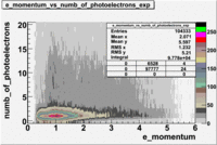
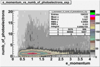
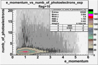
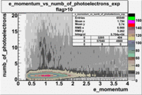
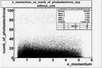
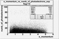
- e_Momentum_vs_Number_of_Photoelectrons
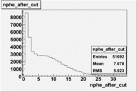
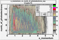
The flag cut applied on the number of photoelectrons means that in CLAS detector instead of 5 superlayers were used 6 of them in track fit. As one can see from the histograms of the Number of photoelectrons, the cut on flag does not have effect on the peak around 1.5phe and decreases the number of entries by 37.17 %. The peak is due to a high energy pions(>2.5GeV), which have enough momentum to emit Cherenkov light and also because of the bad collection of light, there are a particular polar and azimuthal combination of angles where The Cherencov Detector cannot receive emitted light. .
- Number of photoelectrons
| Data | |||
|---|---|---|---|
|
| ||
|
|
Table: Cherenkov fit values
| Distributions | amplitude | mean | width | amplitude | mean | width |
|---|---|---|---|---|---|---|
| without cuts | with cut(flag>10) | |||||
| gauss(0) | p0=2144+/-44.0 | p1=5.342+/-0.343 | p2=7.761+/-0.188 | p0=1580+/-8.1 | p1=3.75+/-0.06 | p2=8.486+/-0.042 |
| landau(3) | p3=4.349e+04+/-2894 | p4=1.049+/-0.026 | p5=0.2197+/-0.0257 | p3=8600+/-3648.7 | p4=-3.861+/-1.414 | p5=-4.88+/-1.41 |
| gauss(6) | p6=4960+/-270.6 | p7=0.7345+/-0.0983 | p8=0.8885+/-0.0594 | p6=6219+/-54.2 | p7=1.088+/-0.006 | p8=0.6037+/-0.0052 |
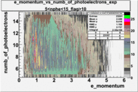
When flag cut(flag>10 cut means that 6 superlayers were used in track fit) was applied the number of entries decreased by 37.17 % and the mean value for the number of photoelectrons is about 7-8. After 5<nphe<15 cut, the number of entries decreased by 66.63 %.The mean value of the nphe is ~9 which agrees with theory(mean value ~13).
| Experiment | B>0 | without cuts | flag>10 | 5<nphe<15 | 5<nphe<15 and flag>10 |
|---|---|---|---|---|---|
|
|
|
|
Pions()
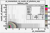
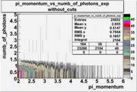
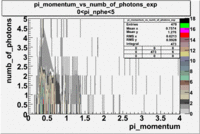
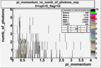
- _Momentum_vs_Number_of_Photons
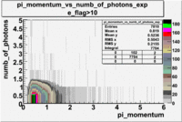
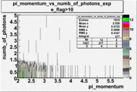
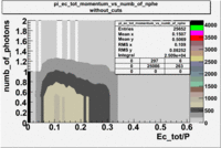
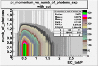
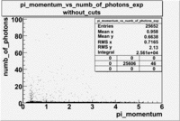
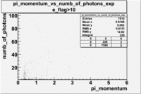
After e_flag>10 cut, the number of entries decreased by 30.45 % and the mean value for the number of photons is ~9
| Experiment | B>0 | without cuts | e_flag>10 | 0<e_nphe<5 | 0<nphe<5 and e_flag>10 |
|---|---|---|---|---|---|
|
|
|
|
Calorimeter
Electron-pion contamination
Osipenko's CLAS Note 2004-20 File:CLAS Note-2004-020.pdf
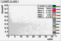
- EC_tot/P_vs_Number_of_Photoelectrons and EC_inner/P_vs_Number_of_Photoelectrons
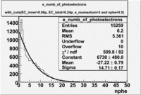
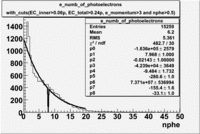
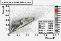
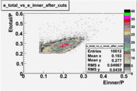
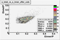
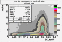
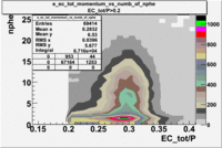
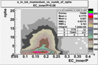
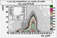
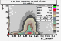
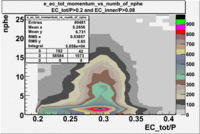
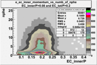
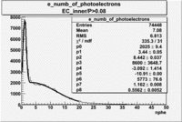
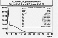
Two types of cuts were applied on the distributions below, one on the energy deposited to the inner calorimeter and another one on the total energy absorbed by the calorimeter , to improve the electron particle identification. In this case was used dst27095_05 file, the beam energy is 5.735 GeV and target NH3.
| without cut | _vs_nphe() | _vs_nphe () | _vs_nphe() |
|---|---|---|---|
|
|
|
|
| _vs_nphe() | _vs_nphe( and ) | _vs_nphe ( and ) |
|---|---|---|
|
|
|
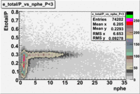
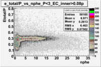
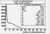
From the EC_tot/P_vs_Number_of_Photoelectrons histogram one can see that the released energy fraction() at ~1.5 nphe peak is much smaller than it should be for electrons. In conclusion, the ~1.5 nphe peak is produced by the tail of negatively charged particles(pions). To eliminate negatively charged pions cut is applied on Calorimeter. After the cut was applied the number of entries decreased by ~33.47%.
Insert example of pion-electron contamination estimate. Use the fits from the cherenkov spectrum to estimate how many pions are stil in the electron sample after the E/P cut.
| with cut() | with cut() | with cuts( and ) | |
|---|---|---|---|
|
|
|
| Distributions | amplitude | mean | width | amplitude | mean | width | amplitude | mean | width |
|---|---|---|---|---|---|---|---|---|---|
| with cut() | with cut() | with cuts( and ) | |||||||
| gauss(0) | p0=1919+/-17.8 | p1=3.593+/-0.233 | p2=8.269+/-0.134 | p0=2025+/-9.4 | p1=3.44+/-0.05 | p2=8.442+/-0.037 | p0=1732+/-8.4 | p1=3.886+/-0.050 | p2=8.069+/-0.037 |
| landau(3) | p3=8600+/-1.4 | p4=-3.063+/-1.414 | p5=-7.138+/-0.000 | p3=8600+/-3648.7 | p4=-3.092+/-1.414 | p5=-10.91+/-0.000 | p3=8600+/-5160.0 | p4=-2.821+/-1.414 | p5=-7.986+/-1.414 |
| gauss(6) | p6=5568+/-69.1 | p7=1.164+/-0.006 | p8=0.543+/-0.008 | p6=5773+/-76.6 | p7=1.162+/-0.008 | p8=0.5562+/-0.0052 | p6=4301+/51.3 | p7=1.189+/-0.008 | p8=0.5299+/-0.0059 |
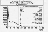
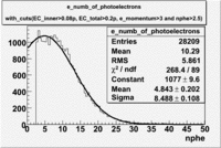
e_numb_of_photoelectrons with the following cuts , . To eliminate the photons produced by the negatively charged pions was used the cut on the momentum e_momentum<3 GeV. Because the high energy pions are able to produce photons, which are misidentified with photoelectrons.
Electron
Cuts
Calorimeter based cuts
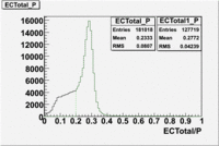
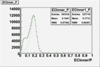
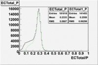
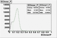
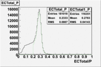
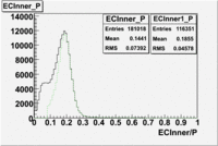
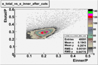
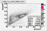
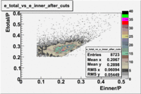
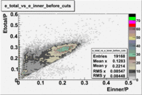
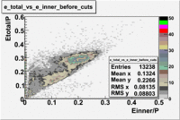
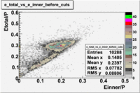
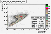
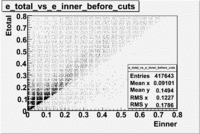
The distributions below represent two types of cuts applied to improve the electron particle identification (PID) using a 4 GeV electron beam incident on an NH3 target. The electron calorimeter is segmented into an inner and an outer region. The total energy absorbed by the calorimeter system is recorded in the variable . The momentum () is calculated using the reconstructed track and the known torus magnetic field. The distributions of and are shown below where both have been divided by the electron momentum and no cuts have been applied.
Without any cuts we have 181018 entries. After using the following cut we are getting 127719 entries, which is about 70.55% of 181018.
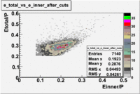
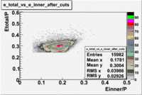
After the cut on the energy deposited into inner part of electron calorimeter, number of entries decreases by 22%.
Both cuts and
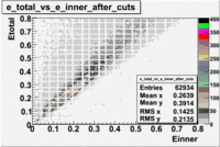
In case of using the cuts of the total deposited energy and the energy deposited into inner calorimeter number of entries decreases ~36%
summary table
The "# of triggers" columns represents the number of events which generated a signal above threshold in the calorimeter and the scintillator. The expected # of events column represents the number of reconstructed events with tracks that also make it through the cuts defined in the table.
The semi-inclusive analysis will focus on the 4 GeV and 6 GeV data which have both inbending and outbending torus settings. Specifically runs 28074 - 28579 ( 4 GeV) and Runs 27356 - 27499 and 26874 - 27198 (6 GeV)
| Beam Energy | Torus Current | Begin Run | End Run | file used | cuts | # trig() | expected # evts() | p<3,,(%) | p>3,,(%) | ||
|---|---|---|---|---|---|---|---|---|---|---|---|
| and | |||||||||||
| 1606 | 1500 | 25488 | 25559 | dst25504_02.B00 | 64% | 49.5% | 78% | 60 | 3.2 | ||
| 1606 | 1946 | 25560 | 25605 | 44 | |||||||
| 1606 | 1500 | 25669 | 25732 | dst25669_02.B00 | 64% | 49% | 78% | 226 | 10 | ||
| 1606 | 1500 | 25742 | 26221 | dst25754_02.B00 | 21% | 11% | 24% | 3154 | 13.3 | ||
| 1606 | -1500 | 26222 | 26359 | dst26224_02.B00 | 4.6% | 3% | 6.6% | 703 | 13.1 | ||
| 1724 | -1500 | 27644 | 27798 | dst27649_02.B00 | 4.8% | 2.2% | 5.9% | 211 | 20 | ||
| 1724 | 1500 | 28512 | 28526 | 159 | |||||||
| 1724 | -1500 | 28527 | 28532 | 93 | |||||||
| 2288 | 1500 | 27205 | 27351 | dst27225_02.B00 | 20.2% | 13% | 25.6% | 1647 | 16.1 | ||
| 2562 | -1500 | 27799 | 27924 | dst27809_02.B00 | 5.7% | 4.6% | 8.6% | 1441 | 13.1 | ||
| 2562 | -1500 | 27942 | 27995 | dst27942_02.B00 | 6.1% | 4.4% | 8.9% | 841 | 32.3 | ||
| 2562 | 1500 | 28001 | 28069 | dst28002_02.B00 | 27.8% | 13% | 29.6% | 1013 | 30.7 | ||
| 2792 | -1500 | 27936 | 27941 | dst27937_02.B00 | 6.7% | 5% | 9.9% | 69 | 20.6 | ||
| 3210 | -2250 | 28549 | 28570 | 436 | |||||||
| 4239 | 2250 | 28074 | 28277 | dst28075_02.B00 | 35.3% | 23.9% | 40.5% | 2278 | 19.6 | ||
| 4239 | -2250 | 28280 | 28479 | dst28281_02.B00 | 9.1% | 9.4% | 13.6% | 2620 | 15.2 | ||
| 4239 | 2250 | 28482 | 28494 | 7 | |||||||
| 4239 | -2250 | 28500 | 28505 | 107 | |||||||
| 4239 | 2250 | 28506 | 28510 | dst28509_02.B00 | 29.5% | 22% | 36% | 75 | 18.1 | ||
| 5627 | 2250 | 27356 | 27364 | dst27358_02.B00 | 33.2% | 27.8% | 41.3% | 56 | 19.4 | 44.6 | 40.1 |
| 5627 | -2250 | 27366 | 27380 | dst27368_02.B00 | 12.6% | 14.8% | 19.5% | 130 | 13.6 | 25.3 | 8.8 |
| 5627 | 2250 | 27386 | 27499 | dst27388_02.B00 | 33.4% | 27.8% | 41.4% | 1210 | 20.2 | 44.8 | 40.1 |
| 5627 | 965 | 27502 | 27617 | 493 | |||||||
| 5735 | -2250 | 26874 | 27068 | dst26904_02.B00 | 13% | 15% | 20% | 1709 | 19.9 | 25.6 | 9.1 |
| 5735 | 2250 | 27069 | 27198 | dst27070_02.B00 | 33.3% | 28.8% | 42.2% | 1509 | 15 | 46 | 40.2 |
| 5764 | -2250 | 26468 | 26722 | dst26489_02.B00 | 12.2% | 14.4% | 19.1% | 1189 | 10 | 24.6 | 9.3 |
| 5764 | 0 | 26723 | 26775 | 268 | |||||||
| 5764 | -2250 | 26776 | 26851 | dst26779_02.B00 | 13.5% | 15.5% | 20.5% | 662 | 15.9 | 26.4 | 9.2 |
Cut on the number of photoelectrons
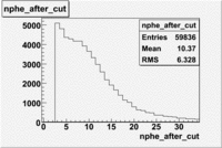
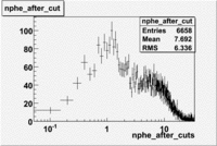
In this case is used a cut on the number of photoelectrons, which is . The plots below show the
effect of the number of photoelectrons cuts on the Cerenkov distribution. We see that after using cut the number of entries decreases ~40.7%
Used cuts and
Used file dst28181_03(energy 4.2GeV). In this case was applied cuts on the polar angle() and momentum(). Number of entries decreased by 96%(?????????????/)
Plot of vs
In this case is used file dst27070(Energy 5.735 GeV and Torus 2250) and are applied the following EC cuts: For ECtotal - , for EC inner - .
P<3
After using above cuts the number of entries decreases ~46%
0.5<P<1
The number of entries decreased by ~51.8%
1<P<1.5
The number of entries decreased approximately by 47.8%
1.5<P<2
In this case the number of entries decreased by 46.1%
2<P<2.5
In this case the number of entries decreased by 38%
P>3
Used file dst27070(Energy 5.735 GeV and Torus 2250) and are applied the following EC cuts: For ECtotal - , for EC inner - .
The number of entries decreased by~40.2%
Plot of EC_tot/P vs nphe for Electrons
Used file dst27070(Energy 5.735 GeV and Torus 2250)
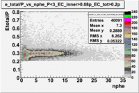
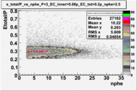
p<3 GeV
The graphs below represents all electron candidates having a momentum smaller than 3 GeV. Negatively charged pions are the most likely particle to be misidentified as an electrons by the tracking software. A negatively charged pion having a momentum of 3 GeV would generate less than ?? photons in the cerenkov counter. As a result the electron candidates which are thought to be misidentified pions. The images which follow represent the effects of several cuts made for the purpose of removing misidentified particles.
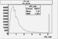
- chi_sqr for pions
- _Momentum_vs_Number_of_Photons for pions()
Used file:27095_05.B00(energy=5.735GeV and torus=2250), everything is done for
p<3 GeV and
p<3 GeV, and
p<3 GeV, , and nphe>2.5
Plot of EC_total vs EC_inner
In this case file dst28181_03.B00 was used(Energy 4.2 GeV and Torus +2250).
The following cuts were applied:, , ec_chi_sqr<0.1 and nphe>3.
Raster and vertex correction
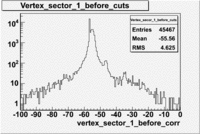
A raster calibration and a cut on the vertex distribution was made in order to select electrons from the polarized target, also the ones scattered from other materials in the beam path. A plot of the uncorrected vertex distribution is presented below for dst27070_02.B00 file(energy=5.7GeV Torus=2250)
Pion
Summary Table
| Beam Energy | Torus Current | Begin Run | End Run | file used | # trig() | expected # evts() | p>3,,(%) | p<3,,(%) |
|---|---|---|---|---|---|---|---|---|
| 1606 | 1500 | 25488 | 25559 | dst25504_02.B00 | 60 | 3.2 | ||
| 1606 | 1500 | 25669 | 25732 | dst25669_02.B00 | 226 | 10 | ||
| 1606 | 1500 | 25742 | 26221 | dst25754_02.B00 | 3154 | 13.3 | ||
| 1606 | -1500 | 26222 | 26359 | dst26224_02.B00 | 703 | 13.1 | ||
| 1724 | -1500 | 27644 | 27798 | dst27649_02.B00 | 211 | 20 | ||
| 2288 | 1500 | 27205 | 27351 | dst27225_02.B00 | 1647 | 16.1 | ||
| 2562 | -1500 | 27799 | 27924 | dst27809_02.B00 | 1441 | 13.1 | ||
| 2562 | -1500 | 27942 | 27995 | dst27942_02.B00 | 841 | 32.3 | ||
| 2562 | 1500 | 28001 | 28069 | dst28002_02.B00 | 1013 | 30.7 | ||
| 2792 | -1500 | 27936 | 27941 | dst27937_02.B00 | 69 | 20.6 | ||
| 4239 | 2250 | 28074 | 28277 | dst28075_02.B00 | 2278 | 19.6 | ||
| 4239 | -2250 | 28280 | 28479 | dst28281_02.B00 | 2620 | 15.2 | ||
| 4239 | 2250 | 28506 | 28510 | dst28509_02.B00 | 75 | 18.1 | ||
| 5627 | 2250 | 27356 | 27364 | dst27358_02.B00 | 56 | 19.4 | 36.1 | 31.5 |
| 5627 | -2250 | 27366 | 27380 | dst27368_02.B00 | 130 | 13.6 | 25 | 43.8 |
| 5627 | 2250 | 27386 | 27499 | dst27388_02.B00 | 1210 | 20.2 | 39.8 | 32.4 |
| 5735 | -2250 | 26874 | 27068 | dst26904_02.B00 | 1709 | 19.9 | 22.5 | 46.4 |
| 5735 | 2250 | 27069 | 27198 | dst27070_02.B00 | 1509 | 15 | 34.6 | 32.9 |
| 5764 | -2250 | 26468 | 26722 | dst26489_02.B00 | 1189 | 10 | 25.2 | 44.3 |
| 5764 | -2250 | 26776 | 26851 | dst26779_02.B00 | 662 | 15.9 | 21.3 | 44 |
Table for Pions
I used the pion id code(both subroutines):
| Beam Energy | Torus Current | Begin Run | End Run | file used | events remaining after cuts | # trig() | expected # evts() | |
|---|---|---|---|---|---|---|---|---|
| first(%) | second(%) | |||||||
| 1606 | 1500 | 25488 | 25559 | dst25504_02.B00 | 96.8 | 99 | 60 | 3.2 |
| 1606 | 1500 | 25669 | 25732 | dst25669_02.B00 | 98.1 | 98.9 | 226 | 10 |
| 1606 | 1500 | 25742 | 26221 | dst25754_02.B00 | 13.4 | 22.8 | 3154 | 13.3 |
| 1606 | -1500 | 26222 | 26359 | dst26224_02.B00 | 11.3 | 15.3 | 703 | 13.1 |
| 1724 | -1500 | 27644 | 27798 | dst27649_02.B00 | 15.3 | 18.7 | 211 | 20 |
| 2288 | 1500 | 27205 | 27351 | dst27225_02.B00 | 16.4 | 18.9 | 1647 | 16.1 |
| 2562 | -1500 | 27799 | 27924 | dst27809_02.B00 | 11.1 | 14.2 | 1441 | 13.1 |
| 2562 | -1500 | 27942 | 27995 | dst27942_02.B00 | 11.1 | 14.2 | 841 | 32.3 |
| 2562 | 1500 | 28001 | 28069 | dst28002_02.B00 | 22.4 | 23.1 | 1013 | 30.7 |
| 2792 | -1500 | 27936 | 27941 | dst27937_02.B00 | 12.3 | 15.4 | 69 | 20.6 |
| 4239 | 2250 | 28074 | 28277 | dst28075_02.B00 | 16.7 | 14.3 | 2278 | 19.6 |
| 4239 | -2250 | 28280 | 28479 | dst28281_02.B00 | 10.4 | 12.6 | 2620 | 15.2 |
| 4239 | 2250 | 28506 | 28510 | dst28509_02.B00 | % | % | 75 | 18.1 |
| 5627 | 2250 | 27356 | 27364 | dst27358_02.B00 | 40.5 | 40.8 | 56 | 19.4 |
| 5627 | -2250 | 27366 | 27380 | dst27368_02.B00 | 9.7 | 12.7 | 130 | 13.6 |
| 5627 | 2250 | 27386 | 27499 | dst27388_02.B00 | 14.1 | 15.5 | 1210 | 20.2 |
| 5735 | -2250 | 26874 | 27068 | dst26904_02.B00 | 12.1 | 14.5 | 1709 | 19.9 |
| 5735 | 2250 | 27069 | 27198 | dst27070_02.B00 | 19.5 | 22.9 | 1509 | 15 |
| 5764 | -2250 | 26468 | 26722 | dst26489_02.B00 | 9.6 | 13.3 | 1189 | 10 |
| 5764 | -2250 | 26776 | 26851 | dst26779_02.B00 | 10.3 | 13.9 | 662 | 15.9 |
Plot of EC_tot/P vs nphe for Pions
Quality Checks
Run Summary Table
The table below uses a characteristic DST file to try and estimate the sample size for a semi-inclusive analysis of pion electroproduction. The column marked "cuts" below indicates the number of events kept when the standard EC based electron identification cuts, described above, are used: and
. The next step will be to compare unpolarized pion production rates in order to evaluate the CLAS detectors efficiencies for measuring charged pions with different torus polarities. The question is whether you get the same rates for negatively charged pions in one torus polarity to positively charged pions using the opposite torus polarity.
| Beam Energy | Torus Current | Target | Begin Run | End Run | file used | # trig() | events remaining after cuts(%) | expected # evts() | events remaining after and cuts(%) | expected # evts() | events remaining after and cuts(%) | expected # evts() |
|---|---|---|---|---|---|---|---|---|---|---|---|---|
| 4239 | 2250 | NH3 | 28205 | 28277 | /cache/mss/home/nguler/dst/dst28205_05.B00 | 1108.72 | 60.8 | 674.1 | 8.3 | 92.02 | 3.24 | 35.92 |
| ND3 | 28074 | 28190 | /cache/mss/home/nguler/dst/dst28187_05.B00 | 1117.87 | 59.6 | 666.25 | 7.99 | 89.32 | 3.3 | 36.9 | ||
| -2250 | NH3 | 28407 | 28479 | /cache/mss/home/nguler/dst/dst28409_05.B00 | 1013.57 | 24.2 | 245.28 | 0.12 | 1.22 | 0 | 0 | |
| ND3 | 28278 | 28403 | /cache/mss/home/nguler/dst/dst28400_05.B00 | 1556.04 | 23.9 | 371.89 | 0.02 | 0.31 | 0.05 | 0.51 | ||
| 5735 | 2250 | NH3 | 27074 | 27195 | /cache/mss/home/nguler/dst/dst27095_05.B00 | 1442.25 | 57.7 | 832.18 | 9.3 | 134.13 | 3.8 | 59.13 |
| ND3 | 27116 | 27170 | /cache/mss/home/nguler/dst/dst27141_05.B00 | 624.55 | 59.1 | 369.10 | 9.53 | 59.52 | 3.9 | 24.36 | ||
| -2250 | NH3 | 26911 | 27015 | /cache/mss/home/nguler/dst/dst26988.B00 | 900.93 | 80.7 | 727.05 | 7.14 | 64.33 | 9.9 | 89.19 | |
| ND3 | 27022 | 27068 | /cache/mss/home/nguler/dst/dst27055_05.B00 | 711.53 | 80 | 569.22 | 6.97 | 49.59 | 10.1 | 71.86 |
Rates
Unpolarized Pion electroproduction
Rates from other experiments in our Kinematic range
Center of Mass Frame Transformation
We have proton and electron. In the Lab frame electron is moving along the x-axis with momentum ; and proton is at rest. The 4-vectors are:
- Lab Frame
- (,,0,0) and for proton :(,0,0,0)
- CM Frame
- :(,,,) and for proton :(,,,)
- Find such that
Using the last two equations we will get the following for x component:
Example of the Missing Mass Calculation for the following reaction
- : electron mass is neglibible
- : Mass of a proton
- Electron
- Proton
- Missing Mass
- Conservation of the 4-momentum gives us following
- Solving it for the final proton state
- In our case 4-vectors for particles are
- Plug and chug
] [ + - -
Example of the Missing Mass Calculation for the following reaction
Used file dst27095_05.B00. Target , Beam Energy 5.735 GeV and Torus Current +2250. Event_number=3106861
- : electron mass is negligible
- : Mass of a proton
- : Mass of a neutron
- Electron
- Neutron
- Missing Mass Calculation
- Below is the conservation of the 4-momentum
- Solving it for the final neutron state
- The 4-vectors for the particles in this event
] [ + - -
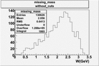
Missing_Mass(experimental data)
The mean value of the missing mass is around 2.056 GeV.
where and - are the 4-momentum of the incident and final electron, - the 4-momentum of the target(proton), - the 4-vector of the .
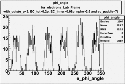
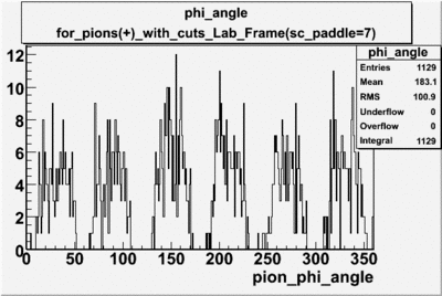
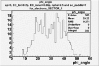
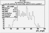
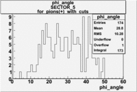
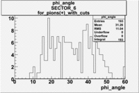
angle
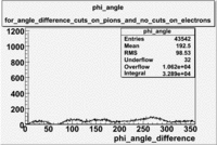
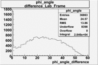
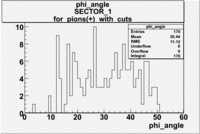
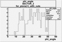
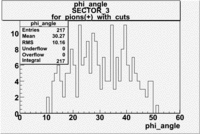
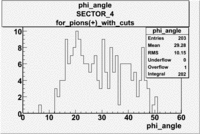
angle for electrons and pions () in lab frame ,
Used file is dst27095_05.B00.Target material is , Torus +2250 and beam energy 5.7 GeV
| For Electrons with cuts (e_p<3, , , nphe>2.5 and sc_paddle=7) | For Pions() with cuts for sc_paddle=7 |
|---|---|
|
|
| For Electrons with cuts (e_p<3, , , nphe>2.5 and sc_paddle=7) | ||
|---|---|---|
| SECTOR 1 | SECTOR 2 | SECTOR 3 |
|
|
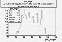
|
| SECTOR 4 | SECTOR 5 | SECTOR 6 |
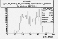
|
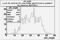
|
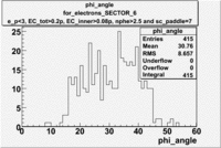
|
| For pions() with cuts for sc_paddle=7 | ||
|---|---|---|
| SECTOR 1 | SECTOR 2 | SECTOR 3 |
|
|
|
| SECTOR 4 | SECTOR 5 | SECTOR 6 |
|
|
|
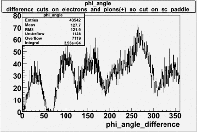
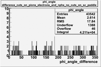
Determine which electron cut is removing the bumps
|
|
Write equation for in terms of Lab frame Momentum and energy.
Graph for Pions hitting paddle #7. The y-axis should be pion counting rate in units of pions per nanCoulomb.
angle in the Center of Mass Frame
The variables below are in Lab Frame:
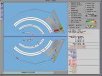
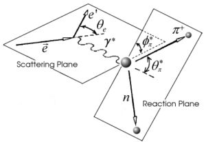
From from CLAS
From the above picture we can write down the momentum x,y and z components for pion in terms of angle and total momentum.
where and are the x and y components of the pion momentum.
The rotation matrix, that rotates the coordinate system around y axis by angle is given
Now, the x, y and z components of the momentum can be written in terms of the momentums of the rotated system.
now rotate about angle
Dr. Forests notes
now rotate about angle
where is the angle between the photon and the electron. The angle can be found using the conservation of momentum and energy.
Conservation of Momentum :
Conservation of Energy :
The can be written in the following way
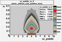
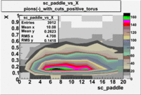
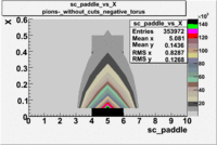
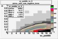
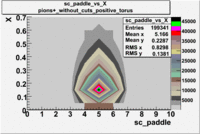
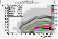
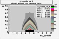
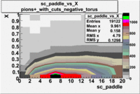
Pion Rates -vs- Paddle for opposite sign Torus fields
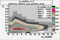
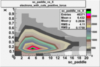
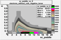
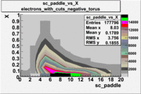
- using all events in which the first particle (the one which caused the trigger) is defined as an electrons and passes the
sc_paddle vs X_bjorken 5.7 GeV Beam Energy
| no cuts | cuts | no cuts | cuts |
|---|---|---|---|
| Electrons | B > 0 | B<0 | |
|
|
|
|
| B > 0 | B<0 | ||
|
|
|
|
| B > 0 | B<0 | ||
|
|
|
|
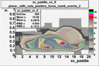
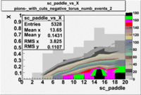
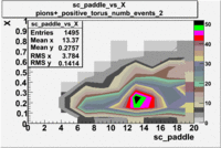
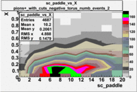
sc_paddle vs X_bjorken with cuts 5.7 GeV Beam Energy(number of events=2)
| B>0 | B<0 |
|
|
| B>0 | B<0 |
|
|
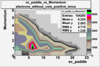
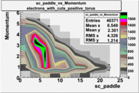
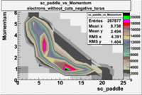
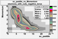
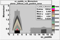
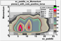
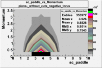
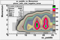
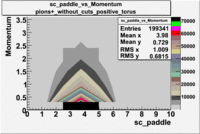
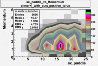
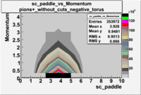
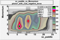
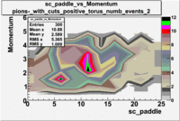
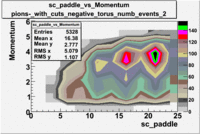
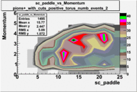
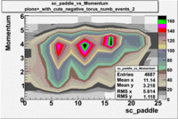
sc_paddle vs Momentum 5.7 GeV Beam Energy
There is a curvature problem.  When B > 0 then I expect the high momentum electrons to hit the lower
paddle numbers   (inbending).   I can see this when I look at the B>0 plot for electrons with cuts.
When B < 0 then the electrons  are bending outwards which makes me expect the the higher momentum
electrons will high the higher numbered paddles.  I do not see this for B>0 with electron cuts.
| no cuts | cuts | no cuts | cuts |
|---|---|---|---|
| Electons | B > 0 | B<0 | |
|
|
|
|
| B > 0 | B<0 | ||
|
 |
|
 |
| B > 0 | B<0 | ||
|
 |
|
 |
sc_paddle vs Momentum with cuts 5.7 GeV Beam Energy(number of events=2)
| B>0 | B<0 |
|
|
| B>0 | B<0 |
|
|
Used file dst26988_05.B00(Energy=5.7GeV and Torus=-2250)
Paddle 7 Rates and statistics
The number of events per trigger is measured for the respective DST file above and then the Total number events in the data set is estimated from that.
| (B>0) | (B<0) | |||
|---|---|---|---|---|
| Total Number Events | Number events per triggers | Total Number Events | Number events per trigger | |
| 0.1 | 5.1 | 71 | 24.6 | 547 |
| 0.2 | 6.9 | 96 | 13.7 | 305 |
| 0.3 | 3.7 | 51 | 6.2 | 137 |
| 0.4 | 3.3 | 45 | 2.7 | 60 |
| 0.5 | 0.9 | 13 | 0.99 | 22 |
Paddle 17 Rates and statistics
| (B<0) | (B>0) | |||
|---|---|---|---|---|
| Total Number Events | Number events per trigger | Total Number Events | Number events per trigger | |
| 0.1 | 6.2 | 137 | 4.6 | 64 |
| 0.2 | 3.5 | 79 | 4.9 | 67 |
| 0.3 | 1.7 | 39 | 2.6 | 36 |
| 0.4 | 0.3 | 7 | 2.1 | 29 |
| 0.5 | 0.1 | 2 | 0.6 | 8 |
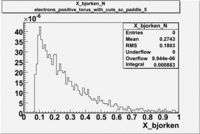
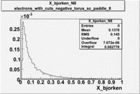
Paddle 5 and 8 Rates and statistics for electrons
| sc_paddle=5 (B>0) | sc_paddle=8 (B<0) | |||
|---|---|---|---|---|
| Total Number Events | Number events per trigger | Total Number Events | Number events per trigger | |
| 0.1 | 384.9 | 5.314 | 1665.2 | 3.706 |
| 0.2 | 382.5 | 5.282 | 977.8 | 2.176 |
| 0.3 | 264.9 | 3.657 | 567.1 | 1.262 |
| 0.4 | 159.5 | 2.202 | 328.6 | 0.7313 |
| 0.5 | 99 | 1.367 | 218.2 | 0.4856 |
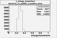
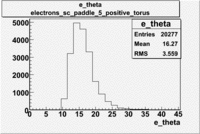
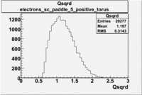
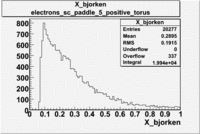
Histograms for 5.7 GeV Beam Energy
| Electron energy/momentum | Electron Theta () | Electron Qsqrd | Electron X_bjorken |
|---|---|---|---|
| B>0 and sc_paddle=5 | |||
|
|
|
|
| B<0 and sc_paddle=8 | |||
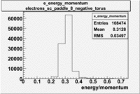
|
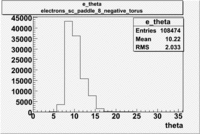
|
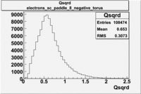
|
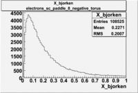
|
Normalized X_bjorken for electrons
| B>0 and sc_paddle=5 | B<0 and sc_paddle=8 |
|---|---|
|
|
Asymmetries
Systematic Errors
Media:SebastianSysErrIncl.pdf Sebastian's Writeup
