Difference between revisions of "LB DetLimits Thesis"
| (50 intermediate revisions by the same user not shown) | |||
| Line 123: | Line 123: | ||
now | now | ||
| − | <math> </math> | + | <math> x = \frac{Y_{2 \sigma}-A}{B} = (0.13 \pm 0.06)\% </math> |
| + | |||
| + | |||
| + | ==Another Method (Se-75)== | ||
| + | For this method, I will use the <math> \frac{A_{Mix}}{a_{Pure}} </math> data and force the activity to be 0 when there is 0% Se in the soil (This was the original goal from gathering the dirt from a national forest) so use the uncorrected concentrations to find how much Se/Soil was "in the dirt to begin with" and force shift the concentration by that amount to force an intercept at (0,0). First, plot the activity ratio as a function of concentration for the previously mentioned ratio. Note the denominator is kept constant, so this plot is measuring how the activity of the mixture behaves. | ||
| + | |||
| + | [[File:A Mix Div a Pure NormCorrected Se75 NoFitRestrict.png|200px]] | ||
| + | |||
| + | Now we have an initial concentration of 0.44%, so shift the concentration by this number | ||
| + | |||
| + | [[File:A Mix Div a Pure NormCorrected Se75 SpikantAdded.png|200px]] | ||
| + | |||
| + | The error in the intercept is high, but it is consistent with zero, so lets increase the intercept by <math> 2 \sigma </math> to get | ||
| + | |||
| + | <math> Y_{2 \sigma} = 0.012289 </math> | ||
| + | |||
| + | Now find the corresponding x point | ||
| + | |||
| + | <math> x = \frac{Y_{2 \sigma} - A}{B} = (0.096 \pm 0.05)\% </math> | ||
| + | |||
| + | This has high error probably due to the uncertainty in the intercept. | ||
| + | |||
| + | ==Another Method (Se-81m)== | ||
| + | Let's repeat this for Se-81m. The plot below will give the initial concentration of Se-81m in the soil. | ||
| + | |||
| + | [[File:A Mix Div a Pure NormCorrected Se81m NoFitRestrict.png|200px]] | ||
| + | |||
| + | The x-intercept is (1.75 +/- 0.17)%, so shift the concentration by this amount. | ||
| + | |||
| + | [[File:A Mix Div a Pure NormCorrected Se81m SpikantAdded.png|200px]] | ||
| + | |||
| + | Now increase the y-intercept by <math> 2 \sigma </math> to get 0.006213, now find the corresponding x-value | ||
| + | |||
| + | <math> x = \frac{Y_{2 \sigma}-A}{B} = (0.42 \pm 0.21)\% </math> | ||
| + | |||
| + | Again this error is high. It would seem plotting the SNR vs. Concentration + Spikant works better | ||
| + | |||
| + | |||
| + | ==X and Y errors (Se-75)== | ||
| + | Now lets repeat the method that yielded the best result, but with x and y errors present. I will be using a TGraphErrors() to plot the data, and fitting with the fit panel. Below is a plot of the activity ratio vs. concentration, but note the errors in x are very small (on the order of 0.05%). | ||
| + | |||
| + | [[File:A Mix Div a Pure NormCorrected Se75 NoFitRestrict XYErrors.png|200px]] | ||
| + | |||
| + | The fit parameters are | ||
| + | |||
| + | Intercept = <math> 5.45571 \times 10^{-2} \pm 0.405627 \times 10^{-2} </math> | ||
| + | |||
| + | Slope = <math> 1.22960 \times 10^{-1} \pm 0.0656862 \times 10^{-1} </math> | ||
| + | |||
| + | The intercept parameter here is slightly different than the fit without the error bars in x. Now find the "initial concentration" | ||
| + | |||
| + | <math> x = \frac{-A}{B} = - \frac{ 5.45571 \times 10^{-2} \pm 0.405627 \times 10^{-2} | ||
| + | }{1.22960 \times 10^{-1} \pm 0.0656862 \times 10^{-1}} = (-0.44 \pm 0.04)\% </math> | ||
| + | |||
| + | This is the same as the above analysis, but I will continue and fix the fit as described above. | ||
| + | |||
| + | [[File:A Mix Div a Pure NormCorrected Se75 FitRestrict XYErrors.png|200px]] | ||
| + | |||
| + | The fit parameters for the fixed fit are | ||
| + | |||
| + | Intercept: <math> 5.45571 \times 10^{-2} \pm 0.405627 \times 10^{-2} </math> | ||
| + | |||
| + | Slope : <math> 5.45500 \times 10^{-1} \pm 4.14090 \times 10^{-5} </math> | ||
| + | |||
| + | Now the "initial concentration" is | ||
| + | |||
| + | <math> x = \frac{-A}{B} = (0.10 \pm 0.01)\% </math> | ||
| + | |||
| + | Now propagate the errors through when shifting the concentration on the signal to noise ratio plot to get accurate x errors. | ||
| + | |||
| + | [[File:N Div B ConcCorrectedbyFix Se75 XYErrors.png|200px]] | ||
| + | |||
| + | The fit parameters are | ||
| + | |||
| + | Intercept: <math> 3.17916 \pm 0.0520972 </math> | ||
| + | |||
| + | Slope: <math> 6.60047 \pm 0.0179356 </math> | ||
| + | |||
| + | which gives a detection limit of <math> 0.016 \pm 0.008 </math> | ||
| + | |||
| + | This is about a factor of 10 worse than before. It could be due to the errors in x pulling the fit upward. The 10% error from shifting the concentration makes the uncertainty higher | ||
| + | |||
| + | Let's try fixing the y-intercept instead, | ||
| + | |||
| + | [[File:A Mix Div a Pure NormCorrected Se75 YintFitRestrict XYErrors.png|200px]] | ||
| + | |||
| + | The new parameters are | ||
| + | |||
| + | Intercept: <math> 1.23 \times 10^{-2} \pm 2.82041 \times 10^{-6} </math> | ||
| + | |||
| + | Slope: <math> 1.52756 \times 10^{-1} \pm 5.91359 \times 10^{-3} </math> | ||
| + | |||
| + | So shift the concentrations over by 0.081 +/- 0.003 | ||
| + | |||
| + | [[File:N Div B ConcCorrectedbyFix Se75 XYErrors YintFix.png|200px]] | ||
| + | |||
| + | |||
| + | After the concentrations have been shifted, the fit parameters are | ||
| + | |||
| + | Intercept: <math> 1.83184 \pm 0.0200626 </math> | ||
| + | |||
| + | Slope: <math> 7.50744 \pm 0.0148123 </math> | ||
| + | |||
| + | which gives a detection limit of (0.005 +/- 0.003)% | ||
| + | |||
| + | ==X and Y Errors (Se-81m)== | ||
| + | Let's repeat the above analysis for Se-81m. First plot the activity ratio as a function of the concentration of Se added to find the "initial concentration" | ||
| + | |||
| + | [[File:A Mix Div a Pure NormCorrected Se81m NoFitRestrict XYErrors.png|200px]] | ||
| + | |||
| + | The fit parameters are | ||
| + | |||
| + | Intercept: <math> 2.59648 \times 10^{-2} \pm 2.05476 \times 10^{-3} </math> | ||
| + | |||
| + | Slope: <math> 1.48111 \times 10^{-2} \pm 7.95127 \times 10^{-4} </math> | ||
| + | |||
| + | which gives an initial concentration of (1.75 +/- 0.17)%. | ||
| + | This is the same as the previous answer, so fix the x-intercept to be less than 0.1% | ||
| + | |||
| + | [[File:A Mix Div a Pure NormCorrected Se81m FitRestrict XYErrors.png|200px]] | ||
| + | |||
| + | The equation of the line is | ||
| + | |||
| + | <math> y(x) = (2.59648 \times 10^{-2} \pm 2.05476 \times 10^{-3}) + (2.59630 \times 10^{-1} \pm 8.52899 \times 10^{-7})x </math> | ||
| + | |||
| + | Now the new x-intercept is (0.1 +/- 0.01)%, now shift the x values and the errors. | ||
| + | |||
| + | |||
| + | The fit parameters become | ||
| + | |||
| + | Intercept: <math> 1.33232 \pm 0.0363379 </math> | ||
| + | |||
| + | Slope: <math> 0.543336 \pm 0.0116317 </math> | ||
| + | |||
| + | [[File:N Div B ConcCorrectedbyFix Se81m XYErrors.png|200px]] | ||
| + | |||
| + | Which gives a detection limit of (0.13 +/- 0.06 )% | ||
| + | |||
| + | Let's try fixing the y-intercept instead of the slope | ||
| + | |||
| + | [[File:A Mix Div a Pure NormCorrected Se81m Yint FitRestrict XYErrors.png|200px]] | ||
| + | |||
| + | The fit parameters are | ||
| + | |||
| + | Intercept: <math> 2.00000 \times 10^{-3} \pm 8.38623 \times 10^{-5} </math> | ||
| + | |||
| + | Slope: <math> 2.02521 \times 10^{-2} \pm 6.43888 \times 10^{-4} </math> | ||
| + | |||
| + | So shift the concentrations over by | ||
| + | |||
| + | <math> 0.099 \pm 0.005 </math> | ||
| + | |||
| + | [[File:N Div B ConcCorrectedbyFix Se81m XYErrors YintFix.png|200px]] | ||
| + | |||
| + | The new fit parameters are | ||
| + | |||
| + | Intercept: <math> 1.33288 \pm 0.0359407 </math> | ||
| + | |||
| + | Slope: <math> 0.543333 \pm 0.0116082 </math> | ||
| + | |||
| + | These parameters give a detection limit of (0.13 +/- 0.06 )% | ||
Latest revision as of 16:40, 6 August 2018
50% Excluded
For this analysis, begin by using the first measurement of the Se-75 line and using the standard exponential decay equation to correct it and its error back to the time of beam off. Below is a table of the Se-75 (120d) corrected measurements as well as the front nickel foils and the Mn-54 data for each measurement. Note the Mn-54 analysis was weighted by the mass of the soil.
| Sample | Activated (total beam time) | Counted | Fully Thesis Corrected Rate @ 1st Measurement (Hz) | |
| 10% Se/Soil Mixture | 5/23/17 and 5/24/17 (83 min) | 07/18/17 (16:25:44) | 3109.68 95.39 | 4280.08 131.29 |
| 10% Se/Soil Pure Witness selenium | 5/23/17 and 5/24/17 (83 min) | 8/1/17 (16:05:51) | 4161.29 127.63 | 6210.50 190.48 |
| 10% Se/Soil Front Inner Ni Foil | 5/23/17 (1h) | 5/23/17 (15:52:21) | 385955 23488.8 | 425064.36 25868.95 |
| 10% Se/Soil Mixture Mn-54 | 5/23/17 (1h) | 07/18/17 (16:25:44) | 15.63 0.56 | 17.67 0.63 |
| 1% Sample Se/Soil Mixture | 5/23/17 (1h) | 6/23/17 (16:39:03) | 2233.33 68.52 | 2675.24 82.08 |
| 1% Sample Se/Soil Pure Witness selenium | 5/23/17 (1h) | 7/20/17 (16:39:46) | 3840.86 117.81 | 5379.43 165.00 |
| 1% Sample Se/Soil Front Inner Ni Foil | 5/23/17 (1h) | 5/23/17 (17:59:39) | 261461 16045.7 | 293170.78 17991.71 |
| 1% Sample Se/Soil Mixture Mn-54 | 5/23/17 (1h) | 6/23/17 (16:39:03) | 9.38 0.39 | 10.05 0.42 |
| 0.1% Sample Se/Soil Mixture | 5/23/17 (30 min) | 6/19/17 (18:25:18) | 849.46 26.07 | 993.59 30.49 |
| 0.1% Sample Se/Soil Pure Witness Selenium | 5/23/17 (30 min) | 07/25/17 (16:32:52) | 834.41 25.61 | 1201.58 36.88 |
| 0.1% Sample Se/Soil Front Inner Ni Foil | 5/23/17 (30 min) | 5/24/17 (14:25:39 | 118412 7280.06 | 197670.18 12152.98 |
| 0.1% Sample Se/Soil Mn-54 | 5/23/17 (30 min) | 6/19/17 (18:25:18) | 9.38 0.33 | 9.96 0.35 |
Mn-54 Efficiency
A calibrated Mn-54 source was used to find the efficiency of an 834 keV line. The source was serial #J4-348, which had an activity of 9.882 on 8/01/12, so the activity on 4/18/17 was
Now converting to Hz gives
| Source | Energy (keV) | Position | Expected Rate (Hz) | ROOT Window (keV) | HpGe Rate (Hz) | HpGe Detector A Efficiency (%) |
| Mn-54 (J4-348) | 834 | 10cm (Det A) | 8138.05 3\% | [829,839] | 25.87 0.28 | 0.32 0.01 |
Activity Ratio Plots (Se-75)
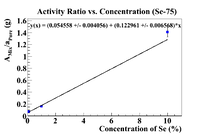
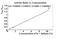
Below are plots of the activity ratio of the Se/Soil mixture and specific activity of the pure selenium pellet as a reference material. The plots also have no restrictions on the equation of the line.
Following the analysis in Nate's thesis, the initial concentration should be the intercept on the x-axis, which is
This is much more physical than previous answers, but I was able to detect Se-75 at a 0.1% level. Let's try some other reference materials
Below is a plot where the activity ratio was taken using Ni-57 as a reference material. This was the front inner Nickel foil
This is not very physical because the graph implies that the initial concentration in the soil was 19.18%, but there were no Se-75 lines observed in a pure soil sample, so this cannot be true
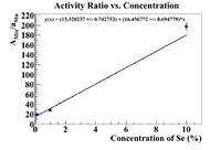
Finally let's try Mn-54 as a reference material as it was internal to the sample.
Now find the initial concentration by finding the x-intercept.
This is still better than the nickel, but still not physical because of the argument presented in the section about the pure selenium ratio.
Now try to fix the linear fit's parameters such that the x-intercept is less than 0.1%. To do this, fix the y-intercept and the slope separately to see if their intercepts agree. If y = A+Bx, when y = 0, then
The fitting function for the plot with the pure selenium used as a reference material was y(x) = (0.054558 +/- 0.004056) + (0.122961 +/- 0.006568)*x, so by fixing the y-intercept, we have
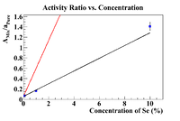
Below is a plot where the red line is the fixed and bounded fit
Even though the y-value was fixed, I kept the error so the fit equation is y(x) = (0.0545580 +/- 0.004056) + (0.545580 +/- 0.0000414)*x, which yields an x intercept of 0.1 +/-0.01 (note that for all plots it seems by bounding the fit the x-intercept will be as close as possible to the closest value before restrictions, so all fixed fits give x-intercepts of 0.1%
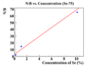
Now shift the concentration values by 0.1%, and plot the signal to noise ratio at the highest measured value.
Now we still have a non-zero y-intercept, but by increasing it by 2 standard deviations gives a value of 0.195189, now finding the value of x for this, we get
where the error is determined by
Where is the y intercept increased by 2 standard deviations
Activity Ratio Plots (Se-81m)
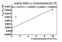
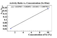
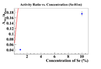
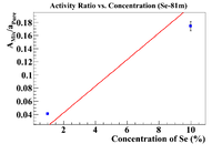
Let's repeat the above analysis with Se-81m data. So begin by plotting the ratio vs the concentration (omitting the 50% sample)
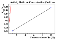
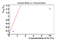
The equation of the fit gives an initial concentration of (1.75 +/- 0.17)%, but I want to force the intercept to be greater than -0.1%, so force the fit to have the desired intercept
Keeping the error in the y-intercept, the equation of the line is
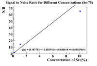
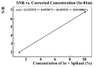
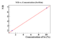
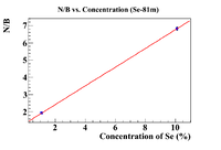
which yields an x-intercept of 0.10000%, so now shift the SNR plot over by 0.1%, and use the values of the highest SNR
now
Another Method (Se-75)
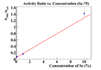
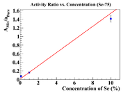
For this method, I will use the data and force the activity to be 0 when there is 0% Se in the soil (This was the original goal from gathering the dirt from a national forest) so use the uncorrected concentrations to find how much Se/Soil was "in the dirt to begin with" and force shift the concentration by that amount to force an intercept at (0,0). First, plot the activity ratio as a function of concentration for the previously mentioned ratio. Note the denominator is kept constant, so this plot is measuring how the activity of the mixture behaves.
Now we have an initial concentration of 0.44%, so shift the concentration by this number
The error in the intercept is high, but it is consistent with zero, so lets increase the intercept by to get
Now find the corresponding x point
This has high error probably due to the uncertainty in the intercept.
Another Method (Se-81m)
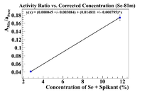
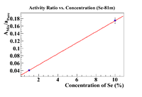
Let's repeat this for Se-81m. The plot below will give the initial concentration of Se-81m in the soil.
The x-intercept is (1.75 +/- 0.17)%, so shift the concentration by this amount.
Now increase the y-intercept by to get 0.006213, now find the corresponding x-value
Again this error is high. It would seem plotting the SNR vs. Concentration + Spikant works better
X and Y errors (Se-75)
Now lets repeat the method that yielded the best result, but with x and y errors present. I will be using a TGraphErrors() to plot the data, and fitting with the fit panel. Below is a plot of the activity ratio vs. concentration, but note the errors in x are very small (on the order of 0.05%).
The fit parameters are
Intercept =
Slope =
The intercept parameter here is slightly different than the fit without the error bars in x. Now find the "initial concentration"
This is the same as the above analysis, but I will continue and fix the fit as described above.
The fit parameters for the fixed fit are
Intercept:
Slope :
Now the "initial concentration" is
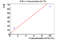
Now propagate the errors through when shifting the concentration on the signal to noise ratio plot to get accurate x errors.
The fit parameters are
Intercept:
Slope:
which gives a detection limit of
This is about a factor of 10 worse than before. It could be due to the errors in x pulling the fit upward. The 10% error from shifting the concentration makes the uncertainty higher
Let's try fixing the y-intercept instead,
The new parameters are
Intercept:
Slope:
So shift the concentrations over by 0.081 +/- 0.003
After the concentrations have been shifted, the fit parameters are
Intercept:
Slope:
which gives a detection limit of (0.005 +/- 0.003)%
X and Y Errors (Se-81m)
Let's repeat the above analysis for Se-81m. First plot the activity ratio as a function of the concentration of Se added to find the "initial concentration"
The fit parameters are
Intercept:
Slope:
which gives an initial concentration of (1.75 +/- 0.17)%. This is the same as the previous answer, so fix the x-intercept to be less than 0.1%
The equation of the line is
Now the new x-intercept is (0.1 +/- 0.01)%, now shift the x values and the errors.
The fit parameters become
Intercept:
Slope:
Which gives a detection limit of (0.13 +/- 0.06 )%
Let's try fixing the y-intercept instead of the slope
The fit parameters are
Intercept:
Slope:
So shift the concentrations over by
The new fit parameters are
Intercept:
Slope:
These parameters give a detection limit of (0.13 +/- 0.06 )%
