LB DetLimits Thesis

50% Excluded

For this analysis, begin by using the first measurement of the Se-75 line and using the standard exponential decay equation to correct it and its error back to the time of beam off. Below is a table of the Se-75 (120d) corrected measurements as well as the front nickel foils and the Mn-54 data for each measurement. Note the Mn-54 analysis was weighted by the mass of the soil.

Sample	Activated (total beam time)	Counted	Fully Thesis Corrected Rate @ 1st Measurement (Hz)	[math] A_{Beam Off} [/math]
10% Se/Soil Mixture	5/23/17 and 5/24/17 (83 min)	07/18/17 (16:25:44)	3109.68 [math] \pm [/math] 95.39	4280.08 [math] \pm [/math] 131.29
10% Se/Soil Pure Witness selenium	5/23/17 and 5/24/17 (83 min)	8/1/17 (16:05:51)	4161.29 [math] \pm [/math] 127.63	6210.50 [math] \pm [/math] 190.48
10% Se/Soil Front Inner Ni Foil	5/23/17 (1h)	5/23/17 (15:52:21)	385955 [math] \pm [/math] 23488.8	425064.36 [math] \pm [/math] 25868.95
10% Se/Soil Mixture Mn-54	5/23/17 (1h)	07/18/17 (16:25:44)	15.63 [math] \pm [/math] 0.56	17.67 [math] \pm [/math] 0.63
1% Sample Se/Soil Mixture	5/23/17 (1h)	6/23/17 (16:39:03)	2233.33 [math] \pm [/math] 68.52	2675.24 [math] \pm [/math] 82.08
1% Sample Se/Soil Pure Witness selenium	5/23/17 (1h)	7/20/17 (16:39:46)	3840.86 [math] \pm [/math] 117.81	5379.43 [math] \pm [/math] 165.00
1% Sample Se/Soil Front Inner Ni Foil	5/23/17 (1h)	5/23/17 (17:59:39)	261461 [math] \pm [/math] 16045.7	293170.78 [math] \pm [/math] 17991.71
1% Sample Se/Soil Mixture Mn-54	5/23/17 (1h)	6/23/17 (16:39:03)	9.38 [math] \pm [/math] 0.39	10.05 [math] \pm [/math] 0.42
0.1% Sample Se/Soil Mixture	5/23/17 (30 min)	6/19/17 (18:25:18)	849.46 [math] \pm [/math] 26.07	993.59 [math] \pm [/math] 30.49
0.1% Sample Se/Soil Pure Witness Selenium	5/23/17 (30 min)	07/25/17 (16:32:52)	834.41 [math] \pm [/math] 25.61	1201.58 [math] \pm [/math] 36.88
0.1% Sample Se/Soil Front Inner Ni Foil	5/23/17 (30 min)	5/24/17 (14:25:39	118412 [math] \pm [/math] 7280.06	197670.18 [math] \pm [/math] 12152.98
0.1% Sample Se/Soil Mn-54	5/23/17 (30 min)	6/19/17 (18:25:18)	9.38 [math] \pm [/math] 0.33	9.96 [math] \pm [/math] 0.35

Mn-54 Efficiency

A calibrated Mn-54 source was used to find the efficiency of an 834 keV line. The source was serial #J4-348, which had an activity of 9.882 [math] \mu Ci [/math] on 8/01/12, so the activity on 4/18/17 was

[math] A(4/18/17) = 9.882 \times e^{-2.57 \times 10^{-8} * 148694400} = 0.22 \mu Ci [/math]

Now converting to Hz gives

[math]\left (0.999760 \right )\left ( 0.22 \times 10^{-6} \mbox{Ci} \right) \left (\frac{ (3.7 \times 10^{10} \mbox{Hz}}{\mbox{Ci}} \right)= (8138.05 \pm 3\%) Hz [/math]

Source	Energy (keV)	Position	Expected Rate (Hz)	ROOT Window (keV)	HpGe Rate (Hz)	HpGe Detector A Efficiency (%)
Mn-54 (J4-348)	834	10cm (Det A)	8138.05 [math] \pm [/math] 3\%	[829,839]	25.87 [math] \pm [/math] 0.28	0.32 [math] \pm [/math] 0.01

Activity Ratio Plots (Se-75)

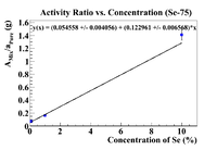
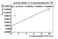
Below are plots of the activity ratio of the Se/Soil mixture and specific activity of the pure selenium pellet as a reference material. The plots also have no restrictions on the equation of the line.

Following the analysis in Nate's thesis, the initial concentration should be the intercept on the x-axis, which is

[math] \frac{0.054558 \pm 0.004056}{0.122961 \pm 0.006568} = (0.44 \pm 0.04)\% [/math]

This is much more physical than previous answers, but I was able to detect Se-75 at a 0.1% level. Let's try some other reference materials

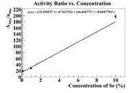
Below is a plot where the activity ratio was taken using Ni-57 as a reference material. This was the front inner Nickel foil

This is not very physical because the graph implies that the initial concentration in the soil was 19.18%, but there were no Se-75 lines observed in a pure soil sample, so this cannot be true

Finally let's try Mn-54 as a reference material as it was internal to the sample.

Now find the initial concentration by finding the x-intercept.

[math] \frac{15.320237 \pm 0.742753}{16.456772 \pm 0.694779} = (0.93 \pm 0.06)\% [/math]

This is still better than the nickel, but still not physical because of the argument presented in the section about the pure selenium ratio.

Now try to fix the linear fit's parameters such that the x-intercept is less than 0.1%. To do this, fix the y-intercept and the slope separately to see if their intercepts agree. If y = A+Bx, when y = 0, then

[math] x = \frac{-A}{B} \gt -0.1 [/math]

The fitting function for the plot with the pure selenium used as a reference material was y(x) = (0.054558 +/- 0.004056) + (0.122961 +/- 0.006568)*x, so by fixing the y-intercept, we have

[math] x=\frac{-0.054558}{B} \gt -0.1, then B\gt 0.54558 [/math]

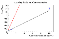
Below is a plot where the red line is the fixed and bounded fit

Even though the y-value was fixed, I kept the error so the fit equation is y(x) = (0.0545580 +/- 0.004056) + (0.545580 +/- 0.0000414)*x, which yields an x intercept of 0.1 +/-0.01 (note that for all plots it seems by bounding the fit the x-intercept will be as close as possible to the closest value before restrictions, so all fixed fits give x-intercepts of 0.1%

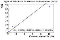
Now shift the concentration values by 0.1%, and plot the signal to noise ratio at the highest measured value.

Now we still have a non-zero y-intercept, but by increasing it by 2 standard deviations gives a value of 0.195189, now finding the value of x for this, we get

[math] x = \frac{y-A}{B} = 0.001 +/- 0.0004 [/math]

where the error is determined by

[math] \sigma_x = \sqrt{(\frac{1}{B})^2 \sigma_A^2 + (\frac{A-Y_{2 \sigma}}{B^2})^2 \sigma_B^2} [/math]