Se170063 Thin Window Analysis

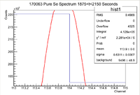
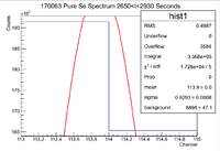
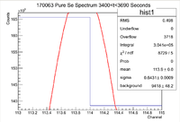
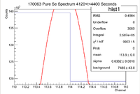
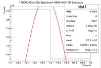
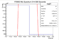
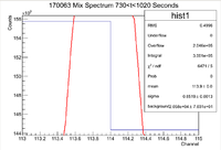
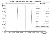
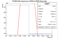
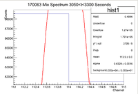
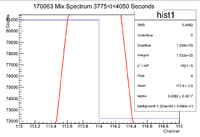
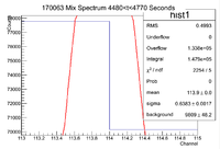
In order to try to pin down the ratio of pure selenium to the selenium in the soil, try using a 2 channel window to find the signal. The error in the signal will be found by integrating the fit gaussian function over the window and "widening" it by half its standard deviation. Since the max value is fixed, it does not appear in the stats box, but I have included it in the table. It would seem that widening the gaussian function by half of its standard deviation yields results that agree up to 3 digits after the decimal with the result of widening the gaussian by its standard deviation. This would imply not much has changed between these methods.

	400 <t< 640 sec	1100 < t < 1360 sec	1875 < t < 2150	2650 < t < 2930 sec	3400 < t < 3690 sec	4120 < t < 4400 sec	4840 < t < 5130 sec
Thin Window
Original Window
Expanded Window
Maximum of Histogram	260980	241756	220348	191476	165549	139528	130930
Original Background	10560 +/- 51.58	10560 +/- 51.41	9496 +/- 48.9	8898 +/- 47.1	9418 +/- 48.2	7485 +/- 43	7032 +/- 31.1
Expanded Background	10750 +/- 42.42	10630 +/- 42.09	9674 +/- 40.2	9029 +/- 38.7	9248 +/- 39.1	7634 +/- 35.5	7161 +/- 34.2
Signal Background (Take Larger Error)	10560 +/- 51.58	10560 +/- 51.41	9496 +/- 48.9	8898 +/- 47.1	9418 +/- 48.2	7485 +/- 43	7161 +/- 34.2
Integrated Background	21120 +/- 103.16	21120 +/- 102.82	18992 +/- 97.8	17796 +/- 94.2	18836 +/- 96.4	14970 +/- 86	14322 +/- 68.4
Signal in Thin Window	466700 +/- 100640	444100 +/- 107283	412800 +/- 105315	356800 +/- 90071	304100 +/- 70533	258700 +/- 63093	233500 +/- 52318
Background Subtracted Signal	445580 +/- 100640	422980 +/- 107283	393808 +/- 105315	339004 +/- 90071	285264 +/- 70533	243730 +/- 63093	219178 +/- 52318
Time Correction Factor (Sec)	400	370	395	400	350	345	360
Corrected Counts	483015.53 +/- 109095.5248	455750 +/- 115595.0622	426463.63 +/- 114048.1804	367485.52 +/- 97638.49218	306127.92 +/- 75691.81615	261292.55 +/- 67639.40782	235683.31 +/- 56257.91145
.dat file entry	7.607165162 +/- 0.2258633895	7.469018062 +/- 0.2536369988	7.346511269 +/- 0.2676838585	7.179649592 +/- 0.2656934406	6.96187741 +/- 0.2472555138	6.838606337 +/- 0.2588646627	6.700363353 +/- 0.2387012956

Below is the table for the Se-Ash Mixture

	0 <t< 300 sec	730 < t < 1020 sec	1480 < t < 1775	2250 < t < 2550 sec	3050< t < 3300 sec	3775 < t < 4050 sec	4480 < t < 4770 sec
Thin Window
Original Window
Expanded Window
Maximum of Histogram	173289	155770	135740	124656	88582	80993	77781
Original Background	29440 +/- 84.93	20580 +/- 70.31	16420 +/- 62.52	14460 +/- 58.47	10950 +/- 50.65	10530 +/- 49.90	9809 +/- 48.2
Expanded Background	28960 +/- 69.12	20580 +/- 57.79	16500 +/- 51.60	14500 +/- 48.2	10630 +/- 41.29	10460 +/- 41.01	9814 +/- 39.7
Signal Background (Take Larger Error)	29440 +/- 84.93	20580 +/- 70.31	16420 +/- 62.52	14460 +/- 58.47	10950 +/- 50.65	10530 +/- 49.90	9809 +/- 48.2
Integrated Background	58880 +/- 169.86	41160 +/- 140.62	32840 +/- 131.04	28920 +/- 116.94	21900 +/- 101.3	21060 +/- 99.8	19618 +/- 96.4
Signal in Thin Window	342200 +/- 92880	300100 +/- 78390	267200 +/- 74626	238600 +/- 63463	170100 +/- 46436	153200 +/- 39780	147900 +/- 38766
Background Subtracted Signal	283320 +/- 92880	258940 +/- 78390	234360 +/- 74626	209680 +/- 63463	148200 +/- 46436.11	132140 +/- 39780.13	128282 +/- 37866.12
.dat file entry	6.850549805 +/- 0.3278271919	6.794470731 +/- 0.3027342241	6.677638317 +/- 0.3181179382	6.549555363 +/- 0.3026659672	6.384857074 +/- 0.3184246458	6.174846148 +/- 0.3010453307	6.092105322 +/- 0.2951787468

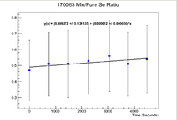
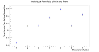
Below is a plot of the ratio of the activities where the pure selenium sample has been time corrected back to match the run time of the mixture.

Note that this does give the expected result that the ratio between the two samples is statistically the same as 0.5, which is the ratio of the masses. The only problem here is that the error is quite large, The average of the uncertainty divided by the mean is 39.6%.

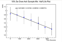
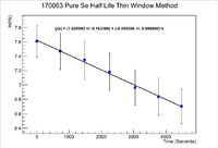
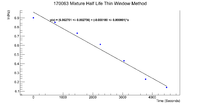
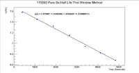
Below are the half life plots for the Pure Selenium sample and the ash mixture

The slope of the mixture plot gives a half life of 63.48 +/- 26.85 minutes. This does overlap, but the error is extremely large.

The slope of the pure selenium sample plot gives a half life of 56.08 +/- 16.33 minutes. Again this does overlap, but the error is still quite large.

The ratio of the initial activities is 0.49 +/- 0.13. Now this does fall within 1 standard deviation of 0.5, which is the value we want.

Dead Time Corrected

I have shown that by tracing the activity back in time for the pure selenium sample that the activities are the same here LB Thesis Thin Window Analysis, but now I must make sure that this will actually give the ratio that is expected.

Begin with the third measurement that was taken for the pure selenium sample

Pure Se Analysis

Third Pure Se Measurement

Below is the histogram of interest

From this we can see that

[math] I \pm \sigma_I = 412800 \pm 642.50 Counts [/math]

and the integrated background is given by

[math] B \pm \sigma_B = 18992 \pm 97.8 Counts[/math]

Now we can find the background subtracted signal

[math] N \pm \sigma_N = 393808 \pm 649.90 Counts[/math]

Now convert this into an activity by dividing by the runtime

[math] A_{Measure} \pm \sigma_{A_{Measure}} = \frac{393808}{275} \pm \frac{649.90}{275} = 1432.03 \pm 2.36 Hz [/math]

Now we can find the true value using the integrated measurement

[math] A_{True} = \frac{e^{\lambda \times 275} \times 1432.03 \times 275 \times \lambda}{e^{\lambda \times 275}-1} = 1472.11 Hz [/math]

[math] \sigma_{A_{True}} = \frac{e^{\lambda \times 275} \times 2.36 \times 275 \times \lambda}{e^{\lambda \times 275}-1} = 2.43 Hz [/math]

So now the true value for the activity is

[math] A_{True} \pm \sigma_{A_{True}} = 1472.11 \pm 2.43 Hz [/math]

Now we must correct for the dead time. The third run had an average count rate of 1387.06 Hz, which corresponds to a dead time of 2.53 +/- 0.3

[math] A_{True}^{DT} = A_{True} \times \frac{1}{1-DT} = 1472.11 \times \frac{1}{0.9747} = 1510.32 Hz [/math]

[math] \sigma_{DTC} = \frac{\sigma_{DT}}{1-DT^2} = 0.003 [/math]

[math] \sigma_{A_{True}^{DT}} = \sqrt{\frac{\sigma_{A_{True}^{DT}}^2}{(1-DT)^2} + \frac{A_{True}^2 \sigma_{DT}^2}{(1-DT)^4}} [/math]

So the real activity for the third measurement of the Pure Se sample is

[math] A_{True}^{DT} \pm \sigma_{A_{True}^{DT}} = 1510.32 \pm 5.08 [/math]

Below is a table representing the numbers that will be put into a data file to be linearly fit (Also using the values from the thesis portion)

Fourth Pure Se Measurement

Now do the analysis for the 4th measurement taken on the pure selenium sample.

Below is the histogram of interest

From this we can see that

[math] I \pm \sigma_I = 356800 \pm 597.33 Counts [/math]

and the integrated background is given by

[math] B \pm \sigma_B = 17796 \pm 94.2 Counts[/math]

Now we can find the background subtracted signal

[math] N \pm \sigma_N = 339004 \pm 604.71 Counts[/math]

Now convert this into an activity by dividing by the runtime

[math] A_{Measure} \pm \sigma_{A_{Measure}} = \frac{339004}{280} \pm \frac{604.71}{280} = 1210.73 \pm 2.16 Hz [/math]

Now we can find the true value using the integrated measurement

[math] A_{True} = \frac{e^{\lambda \times 280} \times 1210.73 \times 280 \times \lambda}{e^{\lambda \times 280}-1} =1245.24 Hz [/math]

[math] \sigma_{A_{True}} = \frac{e^{\lambda \times 280} \times 2.16 \times 280 \times \lambda}{e^{\lambda \times 280}-1} = 2.22 Hz [/math]

So now the true value for the activity is

[math] A_{True} \pm \sigma_{A_{True}} = 1245.24 \pm 2.22 Hz [/math]

Now we must correct for the dead time. The 4th run had an average count rate of 1274.32 Hz, which corr5esponds to a dead time of 2.26 +/- 0.33

[math] A_{True}^{DT} = A_{True} \times \frac{1}{1-DT} = 1245.24 \times \frac{1}{0.9774} = 1274.03 Hz [/math]

[math] \sigma_{DTC} = \frac{\sigma_{DT}}{1-DT^2} = 0.004 [/math]

[math] \sigma_{A_{True}^{DT}} = \sqrt{\frac{\sigma_{A_{True}^{DT}}^2}{(1-DT)^2} + \frac{A_{True}^2 \sigma_{DT}^2}{(1-DT)^4}} [/math]

So the real activity for the third measurement of the Pure Se sample is

[math] A_{True}^{DT} \pm \sigma_{A_{True}^{DT}} = 1274.03 \pm 5.47 [/math]

Fifth Pure Se Measurement

Now do the analysis for the 5th measurement taken on the pure selenium sample.

Below is the histogram of interest

From this we can see that

[math] I \pm \sigma_I = 304100 \pm 551.45 Counts [/math]

and the integrated background is given by

[math] B \pm \sigma_B = 18836 \pm 96.4 Counts[/math]

Now we can find the background subtracted signal

[math] N \pm \sigma_N = 285264 \pm 559.81 Counts[/math]

Now convert this into an activity by dividing by the runtime

[math] A_{Measure} \pm \sigma_{A_{Measure}} = \frac{285264}{290} \pm \frac{559.81}{290} = 983.67 \pm 1.93 Hz [/math]

Now we can find the true value using the integrated measurement

[math] A_{True} = \frac{e^{\lambda \times 290} \times 983.67 \times 290 \times \lambda}{e^{\lambda \times 290}-1} = 1012.72 Hz [/math]

[math] \sigma_{A_{True}} = \frac{e^{\lambda \times 290} \times 1.93 \times 290 \times \lambda}{e^{\lambda \times 290}-1} = 1.99 Hz [/math]

So now the true value for the activity is

[math] A_{True} \pm \sigma_{A_{True}} = 1012.72 \pm 1.99 Hz [/math]

Now we must correct for the dead time. The 5th run had an average count rate of 1168.06 Hz, which corresponds to a dead time of 2.26 +/- 0.33

[math] A_{True}^{DT} = A_{True} \times \frac{1}{1-DT} = 1012.72 \times \frac{1}{0.9774} = 1036.14 Hz [/math]

[math] \sigma_{DTC} = \frac{\sigma_{DT}}{1-DT^2} = 0.003 [/math] [math] \sigma_{A_{True}^{DT}} = \sqrt{\frac{\sigma_{A_{True}^{DT}}^2}{(1-DT)^2} + \frac{A_{True}^2 \sigma_{DT}^2}{(1-DT)^4}} [/math]

So the real activity for the third measurement of the Pure Se sample is

[math] A_{True}^{DT} \pm \sigma_{A_{True}^{DT}} = 1036.14 \pm 3.65 [/math]

Sixth Pure Se Measurement

Now do the analysis for the 6th measurement taken on the pure selenium sample.

Below is the histogram of interest

From this we can see that

[math] I \pm \sigma_I = 258700 \pm 508.63 Counts [/math]

and the integrated background is given by

[math] B \pm \sigma_B = 14970 \pm 86 Counts[/math]

Now we can find the background subtracted signal

[math] N \pm \sigma_N = 243730 \pm 515.85 Counts[/math]

Now convert this into an activity by dividing by the runtime

[math] A_{Measure} \pm \sigma_{A_{Measure}} = \frac{243730}{280} \pm \frac{515.85}{280} = 870.46 \pm 1.84 Hz [/math]

Now we can find the true value using the integrated measurement

[math] A_{True} = \frac{e^{\lambda \times 280} \times 870.46 \times 280 \times \lambda}{e^{\lambda \times 280}-1} = 895.27 Hz [/math]

[math] \sigma_{A_{True}} = \frac{e^{\lambda \times 280} \times 1.84 \times 280 \times \lambda}{e^{\lambda \times 280}-1} = 1.89 Hz [/math]

So now the true value for the activity is

[math] A_{True} \pm \sigma_{A_{True}} = 895.27 \pm 1.89 Hz [/math]

Now we must correct for the dead time. The 6th run had an average count rate of 1168.06 Hz, which corresponds to a dead time of 1.96 +/- 0.26

[math] A_{True}^{DT} = A_{True} \times \frac{1}{1-DT} = 895.27 \times \frac{1}{0.9804} = 913.17 Hz [/math]

[math] \sigma_{DTC} = \frac{\sigma_{DT}}{1-DT^2} = 0.003 [/math] [math] \sigma_{A_{True}^{DT}} = \sqrt{\frac{\sigma_{A_{True}^{DT}}^2}{(1-DT)^2} + \frac{A_{True}^2 \sigma_{DT}^2}{(1-DT)^4}} [/math]

So the real activity for the 6th measurement of the Pure Se sample is

[math] A_{True}^{DT} \pm \sigma_{A_{True}^{DT}} = 913.17 \pm 3.28 [/math]

Seventh Pure Se Measurement

Now do the analysis for the 7th measurement taken on the pure selenium sample.

Below is the histogram of interest

From this we can see that

[math] I \pm \sigma_I = 233500 \pm 483.22 Counts [/math]

and the integrated background is given by

[math] B \pm \sigma_B = 14322 \pm 68.4 Counts[/math]

Now we can find the background subtracted signal

[math] N \pm \sigma_N = 219178 \pm 488.04 Counts[/math]

Now convert this into an activity by dividing by the runtime

[math] A_{Measure} \pm \sigma_{A_{Measure}} = \frac{219178}{290} \pm \frac{488.04}{290} = 755.79 \pm 1.68 Hz [/math]

Now we can find the true value using the integrated measurement

[math] A_{True} = \frac{e^{\lambda \times 290} \times 755.79 \times 290 \times \lambda}{e^{\lambda \times 290}-1} = 778.11 Hz [/math]

[math] \sigma_{A_{True}} = \frac{e^{\lambda \times 290} \times 1.68 \times 290 \times \lambda}{e^{\lambda \times 290}-1} = 1.73 Hz [/math]

So now the true value for the activity is

[math] A_{True} \pm \sigma_{A_{True}} = 778.11 \pm 1.73 Hz [/math]

Now we must correct for the dead time. The 7th run had an average count rate of 1012 Hz, which corresponds to a dead time of 1.96 +/- 0.26

[math] A_{True}^{DT} = A_{True} \times \frac{1}{1-DT} = 778.11 \times \frac{1}{0.9804} = 793.67 Hz [/math]

[math] \sigma_{DTC} = \frac{\sigma_{DT}}{1-DT^2} = 0.003 [/math] [math] \sigma_{A_{True}^{DT}} = \sqrt{\frac{\sigma_{A_{True}^{DT}}^2}{(1-DT)^2} + \frac{A_{True}^2 \sigma_{DT}^2}{(1-DT)^4}} [/math]

So the real activity for the 7th measurement of the Pure Se sample is

[math] A_{True}^{DT} \pm \sigma_{A_{True}^{DT}} = 793.67 \pm 2.92 [/math]

	400 <t< 640 sec	1100 < t < 1360 sec	1875 < t < 2150	2650 < t < 2930 sec	3400 < t < 3690 sec	4120 < t < 4400 sec	4840 < t < 5130 sec
.dat file entry	7.58 +/- 0.003	7.45 +/- 0.003	7.32 +/- 0/003	7.15 +/- 0.004	6.94 +/- 0.004	6.82 +/- 0.004	6.68 +/- 0.004

Se-Sage Mix Analysis

Activity of the First Measurement

Below is the histogram of interest

From this we can see that

[math] I \pm \sigma_I = 342200 \pm 584.98 Counts [/math]

and the integrated background is given by

[math] B \pm \sigma_B = 58880 \pm 169.86 Counts[/math]

Now we can find the background subtracted signal

[math] N \pm \sigma_N = 283320 \pm 609.14 Counts[/math]

Now convert this into an activity by dividing by the runtime

[math] A_{Measure} \pm \sigma_{A_{Measure}} = \frac{283320}{300} \pm \frac{609.14}{300} = 944.4 \pm 2.03 Hz [/math]

Now we can find the true value using the integrated measurement

[math] A_{True} = \frac{e^{\lambda \times 300} \times 944.4 \times 300 \times \lambda}{e^{\lambda \times 300}-1} = 973.26 Hz [/math]

[math] \sigma_{A_{True}} = \sqrt{(\frac{t\times e^{\lambda t} \times \lambda \times \sigma_{A_{Measure}}}{e^{\lambda t}-1})^2 + (\frac{e^{\lambda t}(A t e^{\lambda t} - \lambda^2 - A t + A t \lambda)}{(e^{\lambda t}-1)^2})^2 \times \sigma_{\lambda}^2} = 2.09 Hz [/math]

So now the true value for the activity is

[math] A_{True} \pm \sigma_{A_{True}} =973.26 \pm 2.09 Hz [/math]

Now we must correct for the dead time. The 1st run had an average count rate of 2434.44 Hz, which corresponds to a dead time of 5.06 +/- 0.39

[math] A_{True}^{DT} = A_{True} \times \frac{1}{1-DT} = 944.4 \times \frac{1}{0.9494} = 994.73 Hz [/math]

[math] \sigma_{A_{True}^{DT}} = \sqrt{\frac{\sigma_{A_{True}^{DT}}^2}{(1-DT)^2} + \frac{A_{True}^2 \sigma_{DT}^2}{(1-DT)^4}} [/math]

So the real activity for the 1st measurement of the Mixed sample is

[math] A_{True}^{DT} \pm \sigma_{A_{True}^{DT}} = 994.73 \pm 4.75 [/math]

Activity of the Second Measurement

Below is the histogram of interest

From this we can see that

[math] I \pm \sigma_I = 300100 \pm 547.81 Counts [/math]

and the integrated background is given by

[math] B \pm \sigma_B = 41160 \pm 140.62 Counts[/math]

Now we can find the background subtracted signal

[math] N \pm \sigma_N = 258940 \pm 565.57 Counts[/math]

Now convert this into an activity by dividing by the runtime

[math] A_{Measure} \pm \sigma_{A_{Measure}} = \frac{258940}{290} \pm \frac{547.81}{290} = 892.90 \pm 1.89 Hz [/math]

Now we can find the true value using the integrated measurement

[math] A_{True} = \frac{e^{\lambda \times 290} \times 892.90 \times 290 \times \lambda}{e^{\lambda \times 300}-1} = 919.27 Hz [/math]

[math] \sigma_{A_{True}} = \frac{e^{\lambda \times 290} \times 1.89 \times 290 \times \lambda}{e^{\lambda \times 290}-1} = 1.95 Hz [/math]

So now the true value for the activity is

[math] A_{True} \pm \sigma_{A_{True}} = 919.27 \pm 1.95 Hz [/math]

Now we must correct for the dead time. The 1st run had an average count rate of 1756.30 Hz, which corresponds to a dead time of 3.06 +/- 0.30

[math] A_{True}^{DT} = A_{True} \times \frac{1}{1-DT} = 919.27 \times \frac{1}{0.9694} = 948.29 Hz [/math]

[math] \sigma_{DTC} = \frac{\sigma_{DT}}{1-DT^2} = 0.0.003 [/math] [math] \sigma_{A_{True}^{DT}} = \sqrt{\frac{\sigma_{A_{True}^{DT}}^2}{(1-DT)^2} + \frac{A_{True}^2 \sigma_{DT}^2}{(1-DT)^4}} [/math]

So the real activity for the 2nd measurement of the Mixed sample is

[math] A_{True}^{DT} \pm \sigma_{A_{True}^{DT}} = 948.20 \pm 3.41 [/math]

Activity of the Third Measurement

Below is the histogram of interest

From this we can see that

[math] I \pm \sigma_I = 267200 \pm 516.91 Counts [/math]

and the integrated background is given by

[math] B \pm \sigma_B = 32840 \pm 131.04 Counts[/math]

Now we can find the background subtracted signal

[math] N \pm \sigma_N = 234360 \pm 533.26 Counts[/math]

Now convert this into an activity by dividing by the runtime

[math] A_{Measure} \pm \sigma_{A_{Measure}} = \frac{234360}{295} \pm \frac{533.26}{295} = 794.44 \pm 1.81 Hz [/math]

Now we can find the true value using the integrated measurement

[math] A_{True} = \frac{e^{\lambda \times 295} \times 794.44 \times 295 \times \lambda}{e^{\lambda \times 295}-1} = 818.31 Hz [/math]

[math] \sigma_{A_{True}} = \frac{e^{\lambda \times 295} \times 1.81 \times 295 \times \lambda}{e^{\lambda \times 295}-1} = 1.86 Hz [/math]

So now the true value for the activity is

[math] A_{True} \pm \sigma_{A_{True}} = 818.31 \pm 1.86 Hz [/math]

Now we must correct for the dead time. The 1st run had an average count rate of 1401.98 Hz, which corresponds to a dead time of 2.53 +/- 0.31

[math] A_{True}^{DT} = A_{True} \times \frac{1}{1-DT} = 818.31 \times \frac{1}{0.9747} = 839.55 Hz [/math]

[math] \sigma_{DTC} = \frac{\sigma_{DT}}{1-DT^2} = 0.003 [/math] [math] \sigma_{A_{True}^{DT}} = \sqrt{\frac{\sigma_{A_{True}^{DT}}^2}{(1-DT)^2} + \frac{A_{True}^2 \sigma_{DT}^2}{(1-DT)^4}} [/math]

So the real activity for the 2nd measurement of the Mixed sample is

[math] A_{True}^{DT} \pm \sigma_{A_{True}^{DT}} = 839.55 \pm 3.08 [/math]

Fourth Mix Sample Measurement

Below is the histogram of interest

From this we can see that

[math] I \pm \sigma_I = 238600 \pm 488.47 Counts [/math]

and the integrated background is given by

[math] B \pm \sigma_B = 28920 \pm 116.94 Counts[/math]

Now we can find the background subtracted signal

[math] N \pm \sigma_N = 209680 \pm 502.27 Counts[/math]

Now convert this into an activity by dividing by the runtime

[math] A_{Measure} \pm \sigma_{A_{Measure}} = \frac{209680}{300} \pm \frac{502.27}{300} = 698.93 \pm 1.67 Hz [/math]

Now we can find the true value using the integrated measurement

[math] A_{True} = \frac{e^{\lambda \times 300} \times 698.93 \times 300 \times \lambda}{e^{\lambda \times 300}-1} = 720.29 Hz [/math]

[math] \sigma_{A_{True}} = \frac{e^{\lambda \times 300} \times 1.67 \times 300 \times \lambda}{e^{\lambda \times 300}-1} = 1.72 Hz [/math]

So now the true value for the activity is

[math] A_{True} \pm \sigma_{A_{True}} = 720.29 \pm 1.72 Hz [/math]

Now we must correct for the dead time. The 1st run had an average count rate of 1401.98 Hz, which corresponds to a dead time of 2.53 +/- 0.31

[math] A_{True}^{DT} = A_{True} \times \frac{1}{1-DT} = 720.29 \times \frac{1}{0.9747} = 738.99 Hz [/math]

[math] \sigma_{DTC} = \frac{\sigma_{DT}}{1-DT^2} = 0.003 [/math]

[math] \sigma_{A_{True}^{DT}} = \sqrt{\frac{\sigma_{A_{True}^{DT}}^2}{(1-DT)^2} + \frac{A_{True}^2 \sigma_{DT}^2}{(1-DT)^4}} [/math]>

So the real activity for the 2nd measurement of the Mixed sample is

[math] A_{True}^{DT} \pm \sigma_{A_{True}^{DT}} = 738.99 \pm 2.79 [/math]

Activity of the Fifth Measurement

Below is the histogram of interest

From this we can see that

[math] I \pm \sigma_I = 170100 \pm 412.43 Counts [/math]

and the integrated background is given by

[math] B \pm \sigma_B = 21900 \pm 101.3 Counts[/math]

Now we can find the background subtracted signal

[math] N \pm \sigma_N = 148200 \pm 424.69 Counts[/math]

Now convert this into an activity by dividing by the runtime

[math] A_{Measure} \pm \sigma_{A_{Measure}} = \frac{148200}{250} \pm \frac{424.69}{250} = 592.8 \pm 1.70 Hz [/math]

Now we can find the true value using the integrated measurement

[math] A_{True} = \frac{e^{\lambda \times 250} \times 592.8 \times 250 \times \lambda}{e^{\lambda \times 250}-1} = 607.87 Hz [/math]

[math] \sigma_{A_{True}} = \frac{e^{\lambda \times 250} \times 1.70 \times 250 \times \lambda}{e^{\lambda \times 250}-1} = 1.74 Hz [/math]

So now the true value for the activity is

[math] A_{True} \pm \sigma_{A_{True}} = 607.87 \pm 1.74 Hz [/math]

Now we must correct for the dead time. The 1st run had an average count rate of 1025.13 Hz, which corresponds to a dead time of 1.92 +/- 0.26

[math] A_{True}^{DT} = A_{True} \times \frac{1}{1-DT} = 607.8 \times \frac{1}{0.9808} = 619.70 Hz [/math]

[math] \sigma_{DTC} = \frac{\sigma_{DT}}{1-DT^2} = 0.003 [/math]

[math] \sigma_{A_{True}^{DT}} = \sqrt{DTC^2 \times \sigma_{A}^2 + A^2 \times \sigma_{DTC}^2} = \sqrt{1.02^2 \times 1.74^2 + 607.87^2 \times 0.003^2} = 2.54 Hz [/math]

So the real activity for the 2nd measurement of the Mixed sample is

[math] A_{True}^{DT} \pm \sigma_{A_{True}^{DT}} = 619.70 \pm 2.54 [/math]

Sixth Mix Sample Measurement

Below is the histogram of interest

From this we can see that

[math] I \pm \sigma_I = 153200 \pm 391.41 Counts [/math]

and the integrated background is given by

[math] B \pm \sigma_B = 21060 \pm 99.8 Counts[/math]

Now we can find the background subtracted signal

[math] N \pm \sigma_N = 132140 \pm 403.93 Counts[/math]

Now convert this into an activity by dividing by the runtime

[math] A_{Measure} \pm \sigma_{A_{Measure}} = \frac{132140}{275} \pm \frac{403.93}{275} = 480.51 \pm 1.47 Hz [/math]

Now we can find the true value using the integrated measurement

[math] A_{True} = \frac{e^{\lambda \times 275} \times 480.51 \times 275 \times \lambda}{e^{\lambda \times 275}-1} = 493.96 Hz [/math]

[math] \sigma_{A_{True}} = \frac{e^{\lambda \times 275} \times 1.47 \times 275 \times \lambda}{e^{\lambda \times 275}-1} = 1.51 Hz [/math]

So now the true value for the activity is

[math] A_{True} \pm \sigma_{A_{True}} = 493.96 \pm 1.51 Hz [/math]

Now we must correct for the dead time. The 1st run had an average count rate of 898.19 Hz, which corresponds to a dead time of 1.65 +/- 0.34

[math] A_{True}^{DT} = A_{True} \times \frac{1}{1-DT} = 493.96 \times \frac{1}{0.9835} = 502.25 Hz [/math]

[math] \sigma_{DTC} = \frac{\sigma_{DT}}{1-DT^2} = 0.004 [/math]

[math] \sigma_{A_{True}^{DT}} = \sqrt{DTC^2 \times \sigma_{A}^2 + A^2 \times \sigma_{DTC}^2} = \sqrt{1.02^2 \times 1.51^2 + 493.96^2 \times 0.004^2} = 2.51 Hz [/math]

So the real activity for the 2nd measurement of the Mixed sample is

[math] A_{True}^{DT} \pm \sigma_{A_{True}^{DT}} = 502.25 \pm 2.51 [/math]

Activity of the 7th Measurement

Below is the histogram of interest

From this we can see that

[math] I \pm \sigma_I = 147900 \pm 384.58 Counts [/math]

and the integrated background is given by

[math] B \pm \sigma_B = 19618 \pm 96.4 Counts[/math]

Now we can find the background subtracted signal

[math] N \pm \sigma_N = 128282 \pm 396.48 Counts[/math]

Now convert this into an activity by dividing by the runtime

[math] A_{Measure} \pm \sigma_{A_{Measure}} = \frac{128282}{290} \pm \frac{396.48}{290} = 442.35 \pm 1.38 Hz [/math]

Now we can find the true value using the integrated measurement

[math] A_{True} = \frac{e^{\lambda \times 290} \times 442.35 \times 290 \times \lambda}{e^{\lambda \times 290}-1} = 455.41 Hz [/math]

[math] \sigma_{A_{True}} = \frac{e^{\lambda \times 290} \times 1.38 \times 290 \times \lambda}{e^{\lambda \times 290}-1} = 1.42 Hz [/math]

So now the true value for the activity is

[math] A_{True} \pm \sigma_{A_{True}} = 455.41 \pm 1.42 Hz [/math]

Now we must correct for the dead time. The 1st run had an average count rate of 846.40 Hz, which corresponds to a dead time of 1.65 +/- 0.34

[math] A_{True}^{DT} = A_{True} \times \frac{1}{1-DT} = 455.41 \times \frac{1}{0.9835} = 463.05 Hz [/math]

[math] \sigma_{DTC} = \frac{\sigma_{DT}}{1-DT^2} = 0.004 [/math]

[math] \sigma_{A_{True}^{DT}} = \sqrt{DTC^2 \times \sigma_{A}^2 + A^2 \times \sigma_{DTC}^2} = \sqrt{1.02^2 \times 1.42^2 + 455.41^2 \times 0.004^2} = 2.32 Hz [/math]

So the real activity for the 2nd measurement of the Mixed sample is

[math] A_{True}^{DT} \pm \sigma_{A_{True}^{DT}} = 463.05 \pm 2.32 [/math]

	0<t<300	730 <t< 1020	1480<t<1775	2250<t<2550	3050<t<3300	3775<t<4050	4480<t<4770
Data File Entry	6.90 +/- 0.004	6.85 +/- 0.004	6.73 +/- 0.004	6.61 +/- 0.004	6.43 +/- 0.004	6.23 +/- 0.005	6.14 +/- 0.005

Plots

Below are the time vs. frequency plots

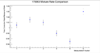
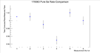
To check consistency I would time correct measurements and take a ratio to compare, for example measurement 1 was taken and a 2nd measurement was taken some time later. So correct the rate of the second measurement back to the first measurement by using the radioactive decay equation, then take a ratio of these 2 numbers.

Another check to do is to take the ratio of the mixture and the pure selenium sample (time corrected to the same time for each measurement) and see if the ratio here is relatively constant

By exponentiating we find that the initial activity of the Mixture is 1056.48 +/- 2.91 Hz, while the pure sample has an initial activity of 2162.90 +/- 5.16 Hz which gives a ratio of

[math] 0.488 \pm 0.002 [/math]

We can also check the ratio of the nickel with the selenium mixture. The rate of the nickel foil was [math] 1.127931 \times 10^6 \pm 7.258 \times 10^3 Hz [/math]

So using the efficiency corrected rate for the soil, we find that the ratio is

[math] 0.134 \pm 0.001 [/math]

The measurement was made 20cm away from the detector face, which has an efficiency of 0.70 +/- 0.0011, so the measurements with the efficiency taken into account are

150925.7143 +/- 392.5923 Hz for the mixture and

308985.7143 +/- 882.6876 Hz for the pure selenium sample