Difference between revisions of "Se170063"
| Line 162: | Line 162: | ||
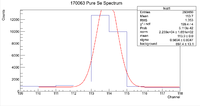
While analyzing the data it became clear that the amplitude of the gaussian fit did not match the amplitude of the peak of interest. Below is an example | While analyzing the data it became clear that the amplitude of the gaussian fit did not match the amplitude of the peak of interest. Below is an example | ||
| + | |||
| + | [[File:170063 PureSeSpectrum HighAmplitude.png|200px]] | ||
| + | |||
| + | This can be corrected in multiple ways. The first way is to use the draw panel to manually adjust the amplitude of the gaussian. The second way (which is the way I used) is to find the maximum value of a histogram in a range of interest using ROOT. | ||
=Runlist= | =Runlist= | ||
Revision as of 16:04, 12 October 2017
PAA_Selenium/Soil_Experiments#Selenium_Sample_Analysis
Sample Description
The sample was placed in an aluminum cylinder that was to be irradiated. The target components consisted of a nickel foil on the front of the cylinder with 2 pure selenium pellets under the foil, but still outside the cylinder. Inside the target there was burnt sagebrush ash, which was burned with a blowtorch, and selenium. Below are the masses of the components
Nickel Foil: 0.2783g
Outer Se Pellets: 0.0971g
Sage Ash: 0.5111g
Inner Se Pellets: 0.0523g
Energy
The Calibration for Detector A was done on the morning of 5/23/17 with the MPA software using the thorium rods (as the calibration was fairly close already) and the correction values were found to be Det A Intercept = -12.208800 slope =1.021270
Efficiency
Nickel Information
Activity and Half Life
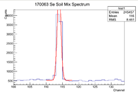
The window used during this investigation was [110,118]. I used the script on daq1 /data/IAC/Se/May2017/5_25_17/Eff.C which fits lines of interest to a Gaussian function plus a constant. Once this function is found, the constant is integrated across the window of interested, then subtracted out of the original equation. After that the Gaussian is integrated across the window which gives the total number of counts for the peak of interest (in this case it is the 93 keV line of Se-81). To find the error in the counts, I increased the value for the standard deviation by a factor of 3 and integrated that function across the region of interest and subtracted that value from the original number of counts. Below is an example of a spectrum seen when using Eff.C
Note that the amplitude of the Gaussian fit is slightly higher than the actual maximum number of counts. To fix this, I simply used ROOT to find the maximum in the given window with
 Int_t max=0;
 hist1->GetXaxis()->SetRange(RangeMin,RangeMax);
 max = hist1 -> GetMaximum();
 cout << "Maximum is     " << max << endl;
After that I forced the amplitude term in the Gaussian to be that maximum via
p0Gauss -> SetParameter(0,max);
Once the raw number of counts and the error has been obtained, before entering the value into a .dat file a few modifications were made to that number. The first and simplest modification is to convert the number of counts into activity simply by dividing by the time duration of the measurement. In other words
Since the radioactive decay equation is given by
So to get a linear equation, simply take the natural log of both sides, which gives
(1)
So we take the natural log of the activity and input that value into the .dat file. To propagate the error we take the error in the number of counts and divide by the time to put the error in units of Hertz. After that, since we are taking the natural log, we must use the standard error propagation formula, which is given by
(2)
Once the activity and its associated error have been computed, put the values into a .dat file with 3 columns. The first column is the time elapsed for the measurement, the second column is the natural log of the activity, and finally the third column is the associated error found as outlined above.
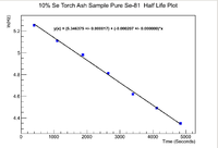
Once the .dat file has been created, simply change the script /data/IAC/Se/May2017/5_25_17/LB_WeightedFit.C to read in the new .dat file and run the script on ROOT. Doing so will give a plot such as the one below
This plot gives parameters of the linear equation (1). The next step in the process is to find the half life of the sample. To do so recall that
Now we must propagate the error in the half life. Even though the error in the decay constant says that it is zero in the plot, by looking at the root output, it can be seen that the error is actually
(See if this can be fixed)
To propagate the error, use the standard propagation of error formula
which gives us a half life of
Minutes
The accepted value of the half life of Se-81 is
Note that these two values do not overlap. This means that there could be some systematic error within the measurement systems.
Now, to find the activity of the sample when it was measured, we use the other parameter given by ROOT. Note that the value given is
This means we must exponentiate to get the initial activity parameter to continue
The associated error to the activity at the time of measurement can be found as well. Since we are exponentiating and the exponential function is its own derivative, the error can be written as
which means that the activity of the Pure Selenium sample at the beginning of the measurement was
Now note that the pure sample was measured second in the split run file. This means that the activity at the beginning of the measurement must be backtracked to when the mixture of ash and selenium was measured, which was 400 seconds prior. To do this, solve the radioactive decay equation for the initial activity.
Now to propagate the error using the standard error propagation formula using 0.5 seconds for the uncertainty in the time.
Which means that the activity of the Pure selenium sample, corrected to be the activity at the same time that the mixture was measure is
Now moving on to the Se-Torch Ash mixture, we can apply a similar analysis to find the initial activity.
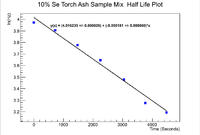
Below is the plot for the half life of the mixture
Now to find the half life use
Propagating the error in the half life gives
Even though the error in the decay constant cannot be seen on the plot, it is given in to ROOT window to be
which mmeans that the half life of the mixed sample is
Now moving on to the activity of the sample. Doing a similar analysis as above we can find the activity of the sample at the beginning of the measurement
and the error is given by
So the activity at the beginning of the measurement is
Now taking the ratio of the activities we get
Alternative Method
While analyzing the data it became clear that the amplitude of the gaussian fit did not match the amplitude of the peak of interest. Below is an example
This can be corrected in multiple ways. The first way is to use the draw panel to manually adjust the amplitude of the gaussian. The second way (which is the way I used) is to find the maximum value of a histogram in a range of interest using ROOT.
Runlist
Table with dates and filename and locations on daq1


