Difference between revisions of "Reconstructing Moller Events"
| (22 intermediate revisions by the same user not shown) | |||
| Line 369: | Line 369: | ||
=Alter Phi Angles= | =Alter Phi Angles= | ||
| − | + | ||
| + | Using the fact that | ||
| + | |||
| + | <center><math>\cos{\phi} \equiv \frac{p_x}{\sqrt{p^2-p_z^2}}</math></center> | ||
| + | |||
| + | |||
| + | <center><math>\Longrightarrow \sqrt{p^2-p_z^2}=\frac{p_x}{\cos{\phi}}=constant</math></center> | ||
| + | |||
| + | |||
| + | We can simply use the expression | ||
| + | |||
| + | <center><math>\frac{p_x}{\cos{\phi}}=\frac{p_x'}{cos{\left(\phi+\delta \phi\right)}}</math></center> | ||
| + | |||
| + | |||
| + | |||
| + | <center><math>\Longrightarrow p_x'=\frac{p_x \times \cos{\left(\phi+\delta \phi\right)}}{\cos{\phi}}</math></center> | ||
| + | |||
| + | |||
| + | Then, using | ||
| + | |||
| + | <center><math>\sqrt{p^2-p_z^2}=\sqrt{p_x^2+p_y^2}</math></center> | ||
| + | |||
| + | |||
| + | <center><math>\Longrightarrow p_y'=\sqrt{p^2-p_z^2-p_x^{'2}}</math></center> | ||
=Run for Necessary Amount to match Cross Section= | =Run for Necessary Amount to match Cross Section= | ||
| − | [[File:MolThetaNH3.png]] | + | <center>[[File:MolThetaNH3.png]]</center> |
Using the above plot for the target material, we can find the relative amount that each Theta angle should observe for this process which gives a known Moller differential cross section. | Using the above plot for the target material, we can find the relative amount that each Theta angle should observe for this process which gives a known Moller differential cross section. | ||
| − | {| border=1 | + | {| class="wikitable" align="center" border=1 |
|- | |- | ||
| − | ! | + | ! Theta (degrees) |
! Number of events | ! Number of events | ||
| Line 415: | Line 438: | ||
|} | |} | ||
| − | We can set up conditional statements to check what range the Theta angle falls in, then by | + | We can set up conditional statements to check what range the Theta angle falls in, then by dividing |
| + | |||
| + | <center><math>\Delta \phi=\frac {2\pi}{number\ of\ events}</math></center> | ||
| + | |||
| + | we should find the change in phi needed to give an evenly distributed distribution around the xy plane for a given Theta angle. | ||
| + | |||
| + | |||
| + | Starting with a data file of momentum components constructed using awk as described above | ||
| + | |||
| + | <center>[[File:Screen_Shot_2016-02-07_at_3.52.37_PM.png | Starting point]]</center> | ||
| + | |||
| + | A program was written to rotate the phi angle as described above. The changing x and y components for this distribution can be seen with | ||
| + | |||
| + | <center>[[File:xy.png]]</center> | ||
| + | |||
| + | Lastly a LUND file was written that was 643360680 lines in length, which equates to 214453560 entries. This was divided into 8579 file parts of 75000 each. The first set from the original data set is shown below. To make sure the full 2 pi is covered, the rotation starts in the 1st quadrant. | ||
| + | |||
| + | <pre>split -a 4 -d -l 75000 Extra_Phi.LUND Phi_Parts_</pre> | ||
| + | |||
| + | |||
| + | <center>[[File:part1of8579.png]]</center> | ||
| − | |||
| − | + | ---- | |
| + | [[DV_MollerTrackRecon#Moller_events_No_Solenoid | Back to Recon ]] | ||
Latest revision as of 00:43, 9 February 2016
Setup
Since we want to run for a evenly spaced energy range for Moller electrons, we will need to use some of the scattered electrons to help cover this range. A Moller scattering data file of 1E7 events has no Moller electrons with momentum over 5500 MeV. Since momentum is conserved, and the data is verified kinematicly verified, we cannot simply "switch" the data. This data can be altered to have a certain number of different phi values for each energy to match the Moller cross section. This data can then be written to a LUND file, and compared to the previous calculations which did not factor in loss of initial energy.
Prepare Data
Using the existing Moller scattering data from a GEANT simulation of 4E7 incident electrons, a file of just scattered momentum components can be constructed using:
awk '{print $9, $10, $11, $16, $17, $18}' MollerScattering_NH3_Large.dat > Just_Scattered_Momentum.dat
Transfer to CM Frame
Center of Mass Frame
4-Momentum Invariants
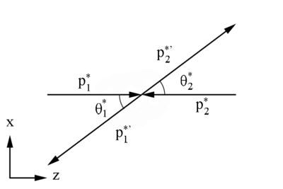
Starting with the definition for the total relativistic energy:
Since we can assume that the frame of reference is an inertial frame, it moves at a constant velocity, the mass should remain constant.
We can use 4-momenta vectors, i.e. ,with c=1, to describe the variables in the CM Frame.
Using the fact that the scalar product of a 4-momenta with itself,
is invariant.
Using this notation, the sum of two 4-momenta forms a 4-vector as well
The length of this four-vector is an invariant as well
Equal masses
For incoming electrons moving only in the z-direction, we can write
We can perform a Lorentz transformation to the Center of Mass frame, with zero total momentum
Without knowing the values for gamma or beta, we can utalize the fact that lengths of the two 4-momenta are invariant
This gives,
Using the fact that
since the rest mass energy of the electrons remains the same in inertial frames.
Substituting, we find
This confirms that the mass remains constant between the frames of reference.
Total Energy in CM
Setting the lengths of the 4-momenta equal to each other,
we can use this for the collision of two particles of mass m. Since the total momentum is zero in the Center of Mass frame, we can express total energy in the center of mass frame as
By the definition of the CM Frame we know
Using the relativistic definition of total energy:
Since the energies are equal, we use this fact to find the momenta
Moller electron Center of Mass Frame
Relativistically, the x and y components remain the same in the conversion from the Lab frame to the Center of Mass frame, since the direction of motion is only in the z direction.
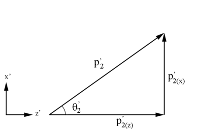
Following the same geometry as for the Lab frame,
Electron Center of Mass Frame
Relativistically, the x, y, and z components have the same magnitude, but opposite direction, in the conversion from the Moller electron's Center of Mass frame to the electron's Center of Mass frame.
where previously it was shown
Determing Angles
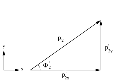
and results based on
Checking on the sign from the cosine results for
We have the limiting range that must fall within:
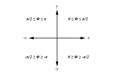
Examining the signs of the components which make up the angle in the 4 quadrants which make up the xy plane:
Partial Check
Alter Phi Angles
Using the fact that
We can simply use the expression
Then, using
Run for Necessary Amount to match Cross Section

Using the above plot for the target material, we can find the relative amount that each Theta angle should observe for this process which gives a known Moller differential cross section.
| Theta (degrees) | Number of events |
|---|---|
| 35 | 130 |
| 30 | 120 |
| 25 | 115 |
| 20 | 100 |
| 15 | 90 |
| 12 | 70 |
| 10 | 60 |
| 8 | 40 |
We can set up conditional statements to check what range the Theta angle falls in, then by dividing
we should find the change in phi needed to give an evenly distributed distribution around the xy plane for a given Theta angle.
Starting with a data file of momentum components constructed using awk as described above

A program was written to rotate the phi angle as described above. The changing x and y components for this distribution can be seen with
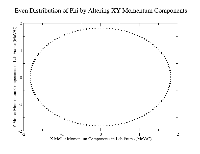
Lastly a LUND file was written that was 643360680 lines in length, which equates to 214453560 entries. This was divided into 8579 file parts of 75000 each. The first set from the original data set is shown below. To make sure the full 2 pi is covered, the rotation starts in the 1st quadrant.
split -a 4 -d -l 75000 Extra_Phi.LUND Phi_Parts_
